Voronoi Diagrams

Definition and Properties

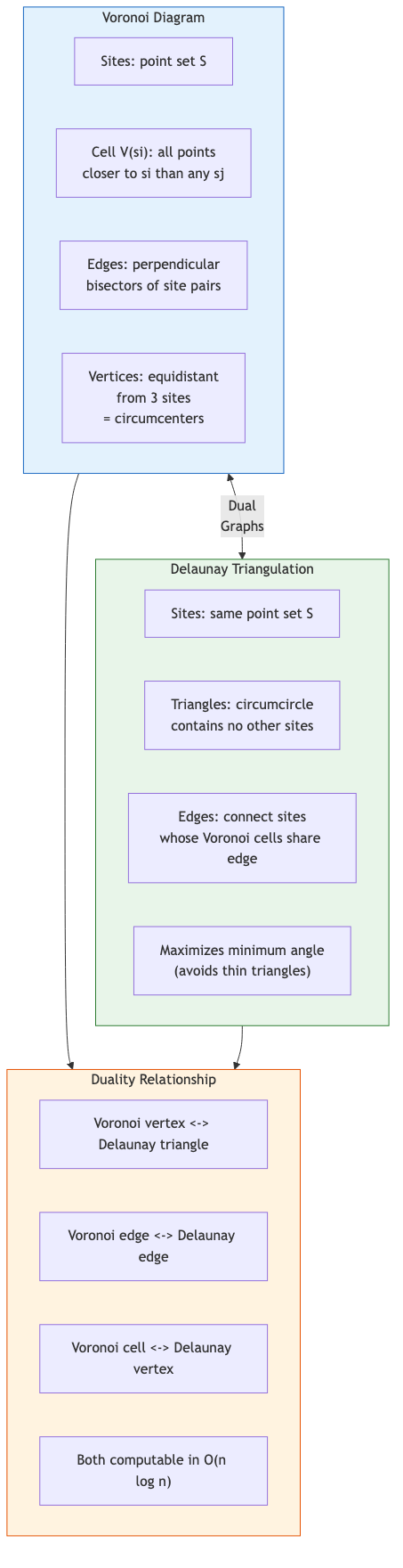
Given a set of $n$ sites $S = \{s_1, \ldots, s_n\}$ in $\mathbb{R}^2$, the Voronoi diagram $\text{Vor}(S)$ partitions the plane into $n$ Voronoi cells, where the cell of $s_i$ is:

$V(s_i) = \{p \in \mathbb{R}^2 : d(p, s_i) \leq d(p, s_j) \text{ for all } j \neq i\}$

Each cell $V(s_i)$ is a (possibly unbounded) convex polygon, being the intersection of $n-1$ halfplanes defined by perpendicular bisectors.

Structural Properties

• Vertices: equidistant from exactly three sites (in general position). A Voronoi vertex is the circumcenter of three sites
• Edges: equidistant from exactly two sites. Each edge lies on the perpendicular bisector of two sites
• Complexity: by Euler's formula, a Voronoi diagram of $n$ sites has at most $2n - 5$ vertices, $3n - 6$ edges, and $n$ faces. This is $O(n)$

Characterization

A point $p$ is a Voronoi vertex iff the largest empty circle centered at $p$ touches three or more sites. A point lies on a Voronoi edge iff the largest empty circle centered at it touches exactly two sites.

The nearest-site Voronoi diagram is the dual of the farthest-site Voronoi diagram (where cells contain points farthest from a given site). The farthest-site Voronoi has cells only for convex hull vertices.

Fortune's Sweep Line Algorithm

Algorithm (Fortune, 1987): $O(n \log n)$ time and $O(n)$ space.

Key idea: sweep a horizontal line downward. The portion of the Voronoi diagram above the sweep line that is determined so far forms a "beach line" --- a sequence of parabolic arcs, each equidistant from a site and the sweep line.

Data structures:

• Beach line: balanced BST storing the sequence of arcs (keyed by $x$-coordinate of intersection with the sweep line). Each arc is defined by a site above the sweep line
• Event queue: priority queue (by $y$-coordinate) storing two types of events

Events:

1. Site event: the sweep line reaches a new site. Insert a new parabolic arc into the beach line (splitting an existing arc). May create new circle event candidates
2. Circle event: three consecutive arcs have their defining sites on a common circle whose lowest point is at the sweep line. The middle arc collapses to a point --- a new Voronoi vertex is created. The arc is removed and adjacent arcs may generate new circle events

Complexity: $O(n)$ site events and $O(n)$ circle events, each processed in $O(\log n)$ time.

Implementation Notes

• Circle events can be false alarms: the middle arc may have been removed before the event fires. Handle by marking events as invalid
• Degenerate cases: cocircular sites (four sites on a circle) produce degree-4 Voronoi vertices; sites at the same $y$-coordinate require careful event ordering
• Numerical precision: circle event detection involves computing circumcenters; use Shewchuk's exact predicates for robustness

Other Construction Algorithms

Divide and Conquer

Shamos and Hoey (1975): $O(n \log n)$

1. Sort sites by $x$-coordinate
2. Recursively compute Voronoi diagrams of left and right halves
3. Merge by computing the dividing chain: a $y$-monotone piecewise-linear curve separating cells belonging to left sites from right sites

The merge step traverses the dividing chain from top to bottom in $O(n)$ time using the structure of the two sub-diagrams.

Incremental Construction

Insert sites one at a time, updating the Voronoi diagram:

• Locate the cell containing the new site: $O(\log n)$ with point location
• The new cell "destroys" portions of neighboring cells
• Expected $O(n \log n)$ with random insertion order (via backward analysis)

Lifting Transform

A deep connection: the Voronoi diagram in $\mathbb{R}^d$ is the projection of the lower convex hull of points lifted to $\mathbb{R}^{d+1}$. Lifting: $(x_1, \ldots, x_d) \mapsto (x_1, \ldots, x_d, \sum x_i^2)$. This transforms Voronoi computation to convex hull computation in one higher dimension.

Applications

Nearest Neighbor Queries

Preprocess $n$ sites into a Voronoi diagram with point location structure. Answer nearest-neighbor queries in $O(\log n)$ time:

1. Locate the Voronoi cell containing the query point
2. The cell's site is the nearest neighbor

Point location via trapezoidal decomposition or Kirkpatrick's hierarchy: $O(n)$ space, $O(\log n)$ query.

Largest Empty Circle

Find the largest circle centered inside a convex region $R$ that contains no sites. The center must be either:

• A Voronoi vertex inside $R$, or
• A point on the boundary of $R$ that is on a Voronoi edge

$O(n \log n)$ algorithm.

Euclidean Minimum Spanning Tree (EMST)

The EMST is a subgraph of the Delaunay triangulation (dual of Voronoi). Algorithm: compute Delaunay triangulation ($O(n \log n)$), then MST of the $O(n)$ Delaunay edges ($O(n \log n)$ total, or $O(n \alpha(n))$ with an optimal MST algorithm on the sparse graph).

Facility Location

The Voronoi diagram provides the partition of customers to nearest facilities. Updating the diagram incrementally supports dynamic facility placement. The farthest-site Voronoi is used for obnoxious facility placement (maximize minimum distance to sites).

Weighted Voronoi Diagrams

Additively Weighted (Johnson-Mehl)

$V_w(s_i) = \{p : d(p, s_i) - w_i \leq d(p, s_j) - w_j \text{ for all } j\}$

Bisectors are hyperbolic arcs (not lines). Cells may be disconnected. Models crystal growth with different start times.

Multiplicatively Weighted (Apollonius)

$V_w(s_i) = \{p : d(p, s_i)/w_i \leq d(p, s_j)/w_j \text{ for all } j\}$

Bisectors are circles (Apollonius circles). Cells are bounded by circular arcs. Used in wireless coverage modeling.

Power Diagram

Each site $s_i$ has weight $w_i$. The power distance from $p$ to $(s_i, w_i)$ is $\|p - s_i\|^2 - w_i$.

$V_\text{pow}(s_i) = \{p : \|p - s_i\|^2 - w_i \leq \|p - s_j\|^2 - w_j \text{ for all } j\}$

Bisectors are lines (affine). The power diagram is an affinely weighted Voronoi diagram and is combinatorially simpler (cells are convex polygons). The dual is the weighted Delaunay triangulation (regular triangulation).

Power diagrams arise in optimal transport (semi-discrete formulation): the optimal assignment of a continuous measure to discrete sinks is given by a power diagram with appropriately chosen weights.

Farthest-Point Voronoi Diagram

$V_\text{far}(s_i) = \{p : d(p, s_i) \geq d(p, s_j) \text{ for all } j\}$

Only convex hull vertices have non-empty cells. Each cell is an unbounded convex region. Complexity: $O(h)$ where $h$ is the hull size.

Application: the smallest enclosing circle has its center at a vertex of the farthest-point Voronoi diagram (or on an edge). $O(n \log n)$ algorithm via the farthest-point Voronoi, though Welzl's randomized algorithm is $O(n)$ expected.

Higher-Order Voronoi Diagrams

The order-$k$ Voronoi diagram partitions the plane into regions where the same $k$ sites are closest:

$V_k(T) = \{p : \max_{s \in T} d(p,s) \leq \min_{s \notin T} d(p,s)\}, \quad |T| = k$

• Complexity: $O(k(n-k))$ regions
• Construction: $O(nk^2 + n \log n)$ or $O(nk \log n)$ via incremental construction
• The order-$k$ Voronoi is the projection of the $k$-level of the lifted arrangement

Applications: $k$-nearest neighbor searching (preprocess for fixed $k$), facility location with backup assignments, interpolation.

Voronoi Diagrams in Higher Dimensions

In $\mathbb{R}^d$, the Voronoi diagram has complexity $O(n^{\lceil d/2 \rceil})$ (can be exponential in $d$). This is the price of the curse of dimensionality.

For $d = 3$: complexity $\Theta(n^2)$ in the worst case. Fortune's sweep generalizes conceptually but is more complex (sweep plane, beach surface of evolving paraboloids).

Practical construction in $\mathbb{R}^3$: incremental algorithms or convex hull in $\mathbb{R}^4$ (via lifting). Libraries: CGAL provides robust 3D Voronoi/Delaunay.

Generalized Voronoi Diagrams

• Voronoi diagram of line segments: sites are line segments. Bisectors are parabolic arcs and line segments. $O(n \log n)$ construction. Used in motion planning, medial axis computation
• Voronoi diagram of convex polygons: more complex bisectors. Applications in robotics (configuration space obstacles)
• Geodesic Voronoi: shortest paths on surfaces instead of Euclidean distance. Used in mesh processing and geographic applications
• Abstract Voronoi diagrams (Klein, 1989): axiomatize the properties needed for Voronoi construction algorithms, yielding a general framework that covers many distance functions