Discrete Fourier Transform
The DFT decomposes a finite signal into its frequency components — the fundamental tool for spectral analysis.
DFT Definition
For a signal x[n] of length N:
X[k] = Σₙ₌₀ᴺ⁻¹ x[n] · e^(-j2πkn/N) k = 0, 1, ..., N-1
Inverse DFT:
x[n] = (1/N) Σₖ₌₀ᴺ⁻¹ X[k] · e^(j2πkn/N) n = 0, 1, ..., N-1
X[k] is a complex number: magnitude |X[k]| = amplitude at frequency k, angle ∠X[k] = phase.
Frequency resolution: Δf = f_s / N. More samples → finer frequency resolution.
Frequency bins: X[k] corresponds to frequency k × f_s / N Hz. X[0] = DC (zero frequency). X[N/2] = Nyquist.
DFT Properties
| Property | Time Domain | Frequency Domain |
|---|---|---|
| Linearity | ax₁[n] + bx₂[n] | aX₁[k] + bX₂[k] |
| Time shift | x[n-m] | X[k] · e^(-j2πkm/N) |
| Frequency shift | x[n] · e^(j2πmn/N) | X[k-m] |
| Circular convolution | x[n] ⊛ h[n] | X[k] · H[k] |
| Parseval's theorem | Σ|x[n]|² | (1/N) Σ|X[k]|² |
Convolution theorem: Circular convolution in time = pointwise multiplication in frequency. This enables fast convolution via FFT.
Fast Fourier Transform (FFT)
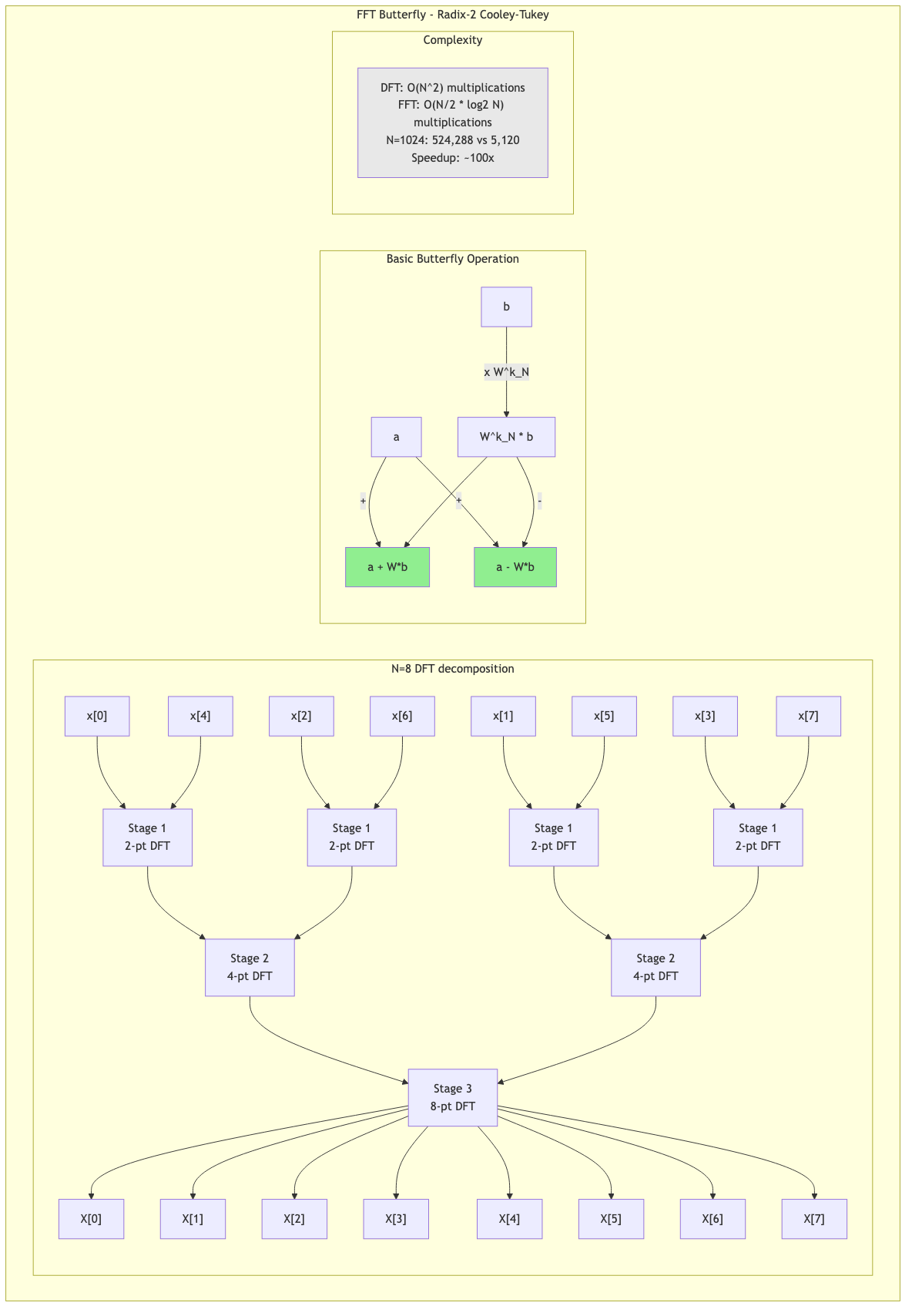
The FFT computes the DFT in O(N log N) instead of O(N²) by exploiting the structure of the DFT matrix.
Cooley-Tukey Algorithm (Radix-2)
Divide and conquer: Split the DFT into even-indexed and odd-indexed samples.
X[k] = Σ x[2m] · W^(2mk) + W^k · Σ x[2m+1] · W^(2mk)
     = DFT_even[k] + W^k · DFT_odd[k]

where W = e^(-j2π/N) (twiddle factor)
Two half-size DFTs + N multiplications and additions → T(N) = 2T(N/2) + O(N) = O(N log N).
Butterfly operation: The basic computational unit:
a' = a + W^k · b
b' = a - W^k · b
PROCEDURE FFT(x)
    n ← LENGTH(x)
    IF n ≤ 1 THEN RETURN

    // Bit-reversal permutation
    j ← 0
    FOR i ← 1 TO n - 1 DO
        bit ← n >> 1
        WHILE (j AND bit) ≠ 0 DO
            j ← j XOR bit
            bit ← bit >> 1
        j ← j XOR bit
        IF i < j THEN SWAP(x[i], x[j])

    // Butterfly stages
    len ← 2
    WHILE len ≤ n DO
        angle ← -2π / len
        wlen ← COMPLEX_FROM_POLAR(1.0, angle)
        FOR i ← 0 TO n - 1 STEP len DO
            w ← COMPLEX(1.0, 0.0)
            FOR j ← 0 TO len/2 - 1 DO
                u ← x[i + j]
                v ← x[i + j + len/2] * w
                x[i + j] ← u + v
                x[i + j + len/2] ← u - v
                w ← w * wlen
        len ← len * 2
Requirement: N must be a power of 2 (pad with zeros if not). Variants exist for arbitrary N (Bluestein, Rader, mixed-radix).
Variants
Radix-4 FFT: Split into 4 groups. Fewer multiplications than radix-2. Used in optimized libraries.
Split-radix FFT: Combine radix-2 and radix-4. Minimum multiplication count.
In-place FFT: Reorder input via bit-reversal permutation, then compute butterflies in place. No extra memory.
Windowing
The DFT assumes the signal is periodic. Discontinuities at the boundaries cause spectral leakage — energy spreads to nearby frequency bins.
Solution: Apply a window function before the DFT to taper the signal smoothly to zero at the boundaries.
| Window | Main Lobe Width | Sidelobe Level | Use |
|---|---|---|---|
| Rectangular | Narrowest (1 bin) | -13 dB | Maximum resolution |
| Hamming | 4 bins | -43 dB | General purpose |
| Hanning (Hann) | 4 bins | -32 dB | General purpose, smooth |
| Blackman | 6 bins | -58 dB | Good sidelobe rejection |
| Kaiser (β) | Variable | Variable | Tunable resolution/leakage |
| Flat-top | 10 bins | -44 dB | Amplitude accuracy |
Tradeoff: Wider main lobe = worse frequency resolution. Lower sidelobes = less leakage. Choose window based on application.
Short-Time Fourier Transform (STFT)
Analyze time-varying frequency content by applying the DFT to windowed segments.
STFT{x}(m, k) = Σₙ x[n] · w[n - m] · e^(-j2πkn/N)
Spectrogram: |STFT|² plotted as a 2D image (time × frequency × magnitude). The standard visualization for audio analysis.
Spectrogram of speech:
Time →
Freq ↑  [formant patterns, harmonics, noise]
Parameters
Window size: Larger → better frequency resolution, worse time resolution.
Hop size: Overlap between windows. Typical: 50-75% overlap.
Time-frequency tradeoff (Heisenberg uncertainty): Cannot have arbitrarily precise time AND frequency resolution simultaneously. Δt × Δf ≥ 1/(4π).
Zero-Padding
Append zeros to the signal before DFT. Does NOT increase frequency resolution (no new information), but increases the number of frequency bins → smoother spectral display (interpolation in frequency).
Useful for: Visualizing spectral peaks more clearly. Matching DFT size to power of 2.
Applications in CS
- Audio processing: Spectrum analysis, pitch detection, equalization, noise reduction, codec design (MP3 uses MDCT, a variant of DFT).
- Image processing: 2D FFT for frequency-domain filtering, JPEG compression (uses DCT, related to DFT).
- Telecommunications: OFDM modulation (Wi-Fi, LTE) — each subcarrier is a frequency bin of the IFFT.
- Scientific computing: Spectral methods for PDEs. Polynomial multiplication via FFT.
- Machine learning: Spectrograms and MFCCs as audio features for speech recognition and music analysis.