
Full-Text Search
Full-text search enables finding documents by their content rather than exact field matches. It powers search boxes across the web, from e-commerce product search to knowledge base lookup, by understanding language structure and relevance.
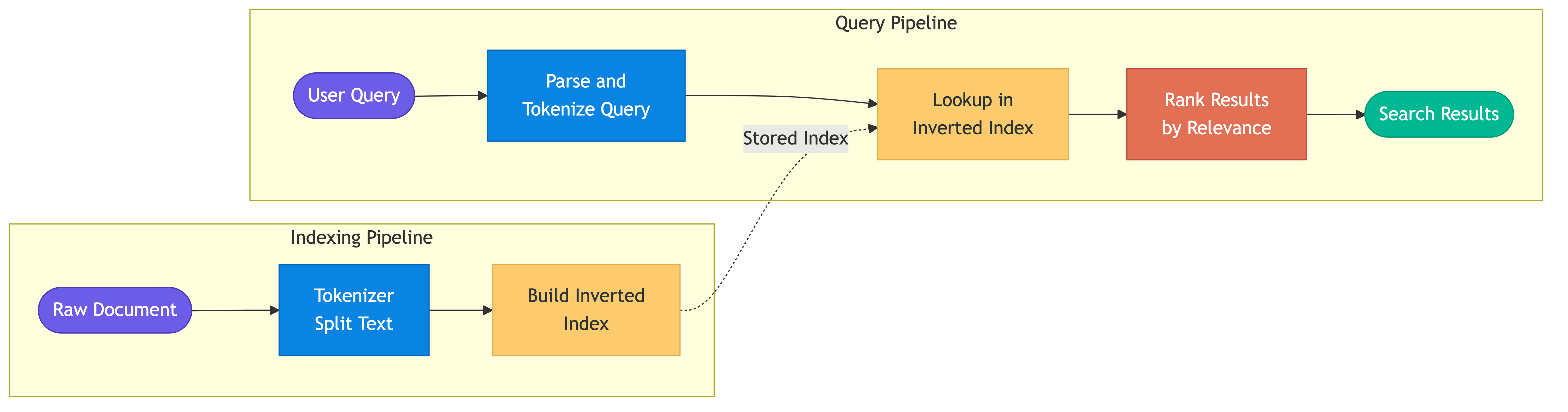
Inverted Indexes
The inverted index is the core data structure behind full-text search. Instead of mapping documents to their words (forward index), it maps each word to the list of documents containing it.
Forward Index vs Inverted Index
Forward index (how documents are stored):
  Doc 1: "the quick brown fox"
  Doc 2: "the lazy brown dog"
  Doc 3: "quick fox jumps"

Inverted index (how search works):
  "the"   --> [Doc 1, Doc 2]
  "quick" --> [Doc 1, Doc 3]
  "brown" --> [Doc 1, Doc 2]
  "fox"   --> [Doc 1, Doc 3]
  "lazy"  --> [Doc 2]
  "dog"   --> [Doc 2]
  "jumps" --> [Doc 3]
Searching for "quick fox" means finding the intersection of the posting lists for "quick" and "fox": documents 1 and 3.
Posting Lists
Each entry in the inverted index points to a posting list containing document IDs, term positions, and term frequencies. Positions enable phrase queries ("quick fox" as an exact phrase vs quick and fox anywhere in the document).
Posting list for "quick":
  Doc 1: positions [2], term_frequency: 1
  Doc 3: positions [1], term_frequency: 1

Phrase query "quick fox":
  "quick" in Doc 1 at position 2, "fox" in Doc 1 at position 4
  Positions are not adjacent --> no phrase match in Doc 1
  "quick" in Doc 3 at position 1, "fox" in Doc 3 at position 2
  Positions are adjacent --> phrase match in Doc 3
Index Segments
Elasticsearch and Lucene use immutable index segments. New documents are written to new segments. Periodically, segments merge. This design enables concurrent reads without locking.
Index lifecycle:
  Write --> in-memory buffer --> flush to new segment (immutable)
  Background: merge small segments into larger ones
  Delete: mark document as deleted (tombstone), removed during merge
Wikipedia's search runs on Elasticsearch with hundreds of millions of documents indexed across sharded, segmented indexes. The immutable segment model enables Wikipedia to handle concurrent searches and article edits without interference.
Tokenization
Tokenization splits text into individual terms (tokens) for indexing. The tokenizer determines what constitutes a searchable unit.
Standard Tokenization
Input: "The user's email is alice@example.com (updated 2025-01-15)"

Whitespace tokenizer:
  ["The", "user's", "email", "is", "alice@example.com", "(updated", "2025-01-15)"]

Standard tokenizer (splits on punctuation and whitespace):
  ["The", "user's", "email", "is", "alice", "example.com", "updated", "2025", "01", "15"]

Custom tokenizer (preserves emails and dates):
  ["The", "user's", "email", "is", "alice@example.com", "updated", "2025-01-15"]
Language-Specific Tokenization
Languages without whitespace delimiters (Chinese, Japanese, Korean) require dictionary-based or statistical segmentation.
Japanese input: "東京都に住んでいます"
Tokenized: ["東京都", "に", "住んで", "います"]

Chinese input: "我在北京工作"
Tokenized: ["我", "在", "北京", "工作"]
Elasticsearch supports language-specific analyzers through plugins like kuromoji (Japanese) and smartcn (Chinese). Google Search handles tokenization across 100+ languages, each with its own linguistic rules.
N-gram Tokenization
N-grams create tokens of fixed character length, useful for partial matching and autocomplete.
Input: "search"
Bigrams (n=2): ["se", "ea", "ar", "rc", "ch"]
Trigrams (n=3): ["sea", "ear", "arc", "rch"]

Edge n-grams (prefix n-grams for autocomplete):
  ["s", "se", "sea", "sear", "searc", "search"]
Stemming & Lemmatization
Stemming and lemmatization reduce words to their root form so that related words match the same index entry.
Stemming
Stemming applies rules to strip suffixes. It is fast but sometimes produces non-words.
Porter Stemmer examples:
  "running"    --> "run"
  "flies"      --> "fli"     (imperfect but consistent)
  "organization" --> "organ" (aggressive, may lose meaning)
  "better"     --> "better"  (no rule applies)
Lemmatization
Lemmatization uses linguistic knowledge to find the dictionary form. More accurate but slower.
Lemmatization examples:
  "running"    --> "run"
  "flies"      --> "fly"     (correct base form)
  "better"     --> "good"    (understands irregular forms)
  "organization" --> "organization" (preserves meaning)
Most production search systems use stemming for speed at index time and query time, accepting the occasional imprecision.
Stop Words
Stop words are common words like "the," "is," "at," and "in" that appear in nearly every document. Historically, search engines removed them to save index space and improve relevance.
Query: "to be or not to be"
After stop word removal: "" (empty query)

Query: "the who"
After stop word removal: "who" (loses the band name)
Modern search engines like Elasticsearch keep stop words in the index but reduce their influence on scoring. This preserves phrase search accuracy while avoiding the relevance noise of ranking by stop word frequency.
TF-IDF
Term Frequency-Inverse Document Frequency is a scoring model that measures how important a word is to a document within a collection.
Term Frequency (TF)
How often a term appears in a document. More occurrences suggest higher relevance.
Document: "the cat sat on the mat. the cat was happy."
TF("cat") = 2 / 10 = 0.2
TF("the") = 3 / 10 = 0.3
TF("happy") = 1 / 10 = 0.1
Inverse Document Frequency (IDF)
How rare a term is across all documents. Rare terms carry more information than common ones.
10,000 documents in the collection:
  "the" appears in 9,800 documents:   IDF = log(10000/9800) = 0.009
  "cat" appears in 500 documents:     IDF = log(10000/500)  = 1.301
  "sphinx" appears in 5 documents:    IDF = log(10000/5)    = 3.301
TF-IDF Score
TF-IDF = TF * IDF

For a document containing "cat" twice in 10 words, across 10,000 docs where "cat" appears in 500:
  TF-IDF("cat") = 0.2 * 1.301 = 0.260

For "the" appearing 3 times:
  TF-IDF("the") = 0.3 * 0.009 = 0.003  (very low, as expected)
TF-IDF correctly ranks documents where rare, specific terms appear frequently as more relevant than documents stuffed with common words.
BM25
BM25 (Best Matching 25) is the evolution of TF-IDF and the default scoring algorithm in Elasticsearch and Lucene. It addresses two key weaknesses of raw TF-IDF.
Term Frequency Saturation
TF-IDF scores increase linearly with term frequency. A document with "cat" 100 times scores 50x higher than one with it twice. BM25 applies a saturation curve so additional occurrences have diminishing returns.
TF-IDF:   score grows linearly with TF
BM25:     score grows quickly at first, then flattens

TF=1:  TF-IDF=1.0   BM25=1.0
TF=2:  TF-IDF=2.0   BM25=1.6
TF=5:  TF-IDF=5.0   BM25=2.3
TF=10: TF-IDF=10.0  BM25=2.7
TF=50: TF-IDF=50.0  BM25=3.0

The k1 parameter controls saturation speed (default: 1.2)
Document Length Normalization
Longer documents naturally contain more term occurrences. BM25 normalizes by document length relative to the average document length in the collection.
BM25 length normalization parameter: b (default: 0.75)
  b=0: no length normalization
  b=1: full length normalization

A 10,000-word document with "cat" appearing 5 times
  is less relevant than a 100-word document with "cat" appearing 5 times.
  BM25 accounts for this; raw TF-IDF does not.
BM25 Formula Summary
BM25(q, d) = sum over query terms t:
  IDF(t) * (TF(t,d) * (k1 + 1)) / (TF(t,d) + k1 * (1 - b + b * |d| / avgdl))

Where:
  TF(t,d) = term frequency of t in document d
  |d|     = document length
  avgdl   = average document length across collection
  k1      = term frequency saturation (default 1.2)
  b       = length normalization (default 0.75)
Elasticsearch defaults to BM25. Amazon product search, GitHub code search, and Stack Overflow all rely on BM25-based scoring as their relevance foundation.
Analyzers & the Indexing Pipeline
The full analysis chain processes text at both index time and query time.
Analysis pipeline:
  Raw text
    --> Character filters (strip HTML, normalize unicode)
    --> Tokenizer (split into tokens)
    --> Token filters (lowercase, stemming, stop words, synonyms)
    --> Indexed terms

Example:
  Input: "<p>The Users' RUNNING shoes</p>"
  Character filter: "The Users' RUNNING shoes"
  Tokenizer: ["The", "Users'", "RUNNING", "shoes"]
  Lowercase: ["the", "users'", "running", "shoes"]
  Stemmer: ["the", "user", "run", "shoe"]
  Stop words: ["user", "run", "shoe"]

  These are the terms stored in the inverted index.
The same analysis chain must run on queries. If "running" is stemmed to "run" at index time but not at query time, the query "running" would not match.
Common Pitfalls
- Mismatched analyzers between index and query time. If you stem at index time, you must stem at query time, or searches will miss documents.
- Over-aggressive stemming. Stemming "university" and "universe" to the same root produces false matches. Test stemmer behavior on your actual content.
- Ignoring language diversity. A single English analyzer fails on multilingual content. Detect language per document and apply appropriate analyzers.
- Indexing everything as keyword fields. Keyword fields support exact match only, not full-text search. Use text fields with analyzers for searchable content.
- Not tuning BM25 parameters. The defaults work well for general text, but short documents (tweets, product titles) benefit from adjusting k1 and b.
- Treating search as a simple database query. Full-text search is probabilistic ranking, not exact matching. Users expect fuzzy, forgiving results.
Key Takeaways
- The inverted index maps terms to documents, enabling fast full-text lookup. It is the foundation of every search engine.
- Tokenization, stemming, and stop word handling must be consistent between index time and query time.
- BM25 improves on TF-IDF by adding term frequency saturation and document length normalization. It is the default relevance model in modern search engines.
- The analysis pipeline (character filters, tokenizer, token filters) determines what is searchable. Misconfigured analyzers are the most common source of "search is broken" bugs.
- Full-text search is about relevance ranking, not exact matching. Invest in understanding your scoring model before reaching for complex customizations.