Self-Supervised Learning

Overview

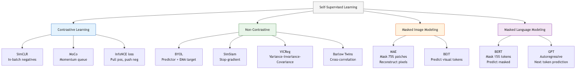
Self-Supervised Learning Methods Overview

Self-supervised learning (SSL) learns representations from unlabeled data by solving pretext tasks — tasks derived from the data's own structure. The goal is to learn general-purpose features that transfer to downstream tasks with limited labeled data. SSL has closed (and sometimes surpassed) the gap between supervised and unsupervised learning in vision, NLP, and other domains.

Why Self-Supervision?

Labeled data is expensive and domain-specific. Unlabeled data is abundant. SSL exploits the structure of unlabeled data (spatial, temporal, semantic) to learn representations capturing meaningful patterns. The learned features serve as initialization for downstream tasks (fine-tuning) or directly as frozen features (linear probing).

Contrastive Learning

Core Principle

Learn an embedding space where positive pairs (different views of the same instance) are pulled together and negative pairs (views of different instances) are pushed apart. The InfoNCE loss (van den Oord et al., 2018):

L = -log [exp(sim(z_i, z_j^+)/τ) / Σ_k exp(sim(z_i, z_k)/τ)]

where sim is cosine similarity, τ is a temperature parameter, z_j^+ is the positive pair, and the sum in the denominator includes one positive and many negatives. This loss is a lower bound on the mutual information between the views.

SimCLR

Chen et al. (2020) established the modern contrastive learning recipe:

Data augmentation: Apply two random augmentations (crop, color jitter, Gaussian blur, horizontal flip) to each image, creating a positive pair.
Encoder: A backbone network (ResNet-50) maps augmented views to representations h = f(x).
Projection head: A small MLP maps h to z = g(h) where the contrastive loss is applied. Crucially, the projection head is discarded after pretraining — h (not z) is used for downstream tasks.
Loss: InfoNCE over all pairs in the mini-batch. Negative pairs are all other images in the batch.

Key findings: Large batch sizes (4096-8192) are critical for sufficient negatives. Strong augmentation (especially color jitter) is essential. The projection head is vital — contrastive loss in z space learns better h representations than directly in h space.

SimCLR v2: Adds a deeper projection head (3-layer MLP), momentum encoder, and self-distillation with a larger teacher model. Achieves strong semi-supervised performance.

MoCo (Momentum Contrast)

He et al. (2020) decouple the negative sample pool from the batch size using a memory queue:

A query encoder processes the current view: q = f_q(x^q).
A key encoder (momentum-updated copy of the query encoder) processes augmented views and fills a queue: k = f_k(x^k).
The queue stores recent key embeddings as negatives (65536 keys), independent of batch size.
Momentum update: θ_k ← m·θ_k + (1-m)·θ_q, with m = 0.999.

The momentum encoder provides a slowly-evolving representation for consistent negatives, avoiding the need for large batches.

MoCo v2: Adopts SimCLR's stronger augmentation and projection head. MoCo v3 (2021): Applies to Vision Transformers (ViT), drops the queue, uses high momentum.

BYOL (Bootstrap Your Own Latent)

Grill et al. (2020) achieved strong SSL without negative pairs. Architecture:

Online network: encoder + projector + predictor → p = predict(project(encode(x₁)))
Target network: encoder + projector (momentum-updated) → z = project(encode(x₂))
Loss: L = -2 · sim(p, sg(z)) (stop-gradient on target)

The predictor MLP (asymmetry between online and target) plus momentum update prevents representation collapse (all inputs mapping to the same point). Without these, minimizing similarity between positive pairs alone would trivially collapse to a constant.

Why it works: The momentum target provides a slowly-moving regression target. The predictor must learn to anticipate the target's representation, which requires encoding meaningful information. Information-theoretic analyses show BYOL implicitly maximizes an information-theoretic objective.

Masked Prediction

Masked Image Modeling

Inspired by BERT's masked language modeling, masked image modeling (MIM) masks portions of the input image and trains the model to reconstruct them.

MAE (Masked Autoencoder)

He et al. (2022) mask a high percentage (75%) of image patches and train a ViT to reconstruct the masked pixels:

Encoding: Only visible (unmasked) patches are fed to the encoder (efficiency gain).
Decoding: A lightweight decoder takes encoded visible patches plus mask tokens and reconstructs all patches.
Loss: MSE on pixel values of masked patches only.

Key insight: The high masking ratio (75%) creates a non-trivial prediction task that forces the encoder to learn semantic representations. Low masking ratios allow trivial interpolation.

Efficiency: Processing only 25% of patches makes the encoder 3-4x faster than processing all patches. The decoder is small (shallow transformer), so total training cost is reduced.

BEiT

Bao et al. (2022) use a discrete visual tokenizer (from DALL-E's VQ-VAE) to convert image patches to visual tokens. The MIM pretext task predicts the visual token (categorical cross-entropy) of masked patches rather than raw pixels. This provides a more semantic target than pixel reconstruction.

BEiT v2: Uses a learned visual tokenizer (VQ-KD) distilled from a CLIP-pretrained teacher, producing more semantically meaningful tokens.

DINO and DINOv2

DINO (Self-Distillation with No Labels)

Caron et al. (2021) train ViTs via self-distillation:

Student: Processes local crops (small random crops) and global crops.
Teacher: Processes only global crops. Updated via EMA of student weights.
Loss: Cross-entropy between student and teacher softmax outputs (with centering and sharpening to prevent collapse).

Emergent properties: DINO-trained ViTs exhibit remarkable properties — the self-attention maps in the last layer explicitly segment objects without any segmentation supervision. The [CLS] token captures semantic structure; k-NN classification on frozen features achieves strong results without fine-tuning.

DINOv2

Ousterhout et al. (2023) scale DINO to produce general-purpose visual features:

Curated pretraining data: Large, curated dataset (LVD-142M) using automated pipeline for deduplication and quality filtering.
Combine objectives: DINO self-distillation + iBOT (masked image modeling) jointly.
Scale: ViT-g (1.1B parameters) with KD to smaller models.
Result: Frozen DINOv2 features match or exceed task-specific fine-tuned models on many benchmarks (depth estimation, segmentation, classification) without any task-specific training.

I-JEPA (Image-based Joint-Embedding Predictive Architecture)

Assouline et al. (2023) predict abstract representations of masked regions (not pixels):

A context encoder processes visible patches.
A predictor takes context representations and mask token positions to predict the target representations (from a momentum-updated target encoder) of masked patches.
Loss is in representation space (L2 between predicted and target representations).

Key difference from MAE: Predicts in representation space, not pixel space. This avoids learning low-level texture details and focuses on semantic content. No decoder needed for pixel reconstruction.

Difference from contrastive methods: No negative pairs, no hand-crafted augmentations (only masking). The prediction task itself provides the learning signal.