Probability Distributions
This file catalogs the major probability distributions, their properties, relationships, and applications. Distributions covered in the discrete math probability file are revisited here with more depth.
Discrete Distributions
Bernoulli(p)
Single binary trial. X ∈ {0, 1}.
P(X = 1) = p,  P(X = 0) = 1 - p = q
E[X] = p,  Var(X) = pq
MGF: M(t) = q + pe^t
Binomial(n, p)
Number of successes in n independent Bernoulli(p) trials.
P(X = k) = C(n,k) p^k q^(n-k),  k = 0,...,n
E[X] = np,  Var(X) = npq
MGF: M(t) = (q + pe^t)^n
Sum of n independent Bernoulli(p) variables. Normal approximation: X ≈ N(np, npq) when np ≥ 5 and nq ≥ 5. Poisson approximation: X ≈ Poisson(np) when n is large and p is small.
Geometric(p)
Number of trials until first success.
P(X = k) = q^(k-1) p,  k = 1, 2, ...
E[X] = 1/p,  Var(X) = q/p²
Memoryless: P(X > s+t | X > s) = P(X > t). The only discrete memoryless distribution.
Alternative form: number of failures before first success (starts at 0).
Negative Binomial(r, p)
Number of trials until the r-th success.
P(X = k) = C(k-1, r-1) p^r q^(k-r),  k = r, r+1, ...
E[X] = r/p,  Var(X) = rq/p²
Sum of r independent Geometric(p) variables. Geometric is a special case (r = 1).
Hypergeometric(N, K, n)
Drawing n items without replacement from N items containing K successes.
P(X = k) = C(K,k) C(N-K, n-k) / C(N, n)
E[X] = nK/N,  Var(X) = n(K/N)(1-K/N)(N-n)/(N-1)
Like Binomial but without replacement. Approaches Binomial as N → ∞.
Application: Quality control (defective items in a sample), Fisher's exact test.
Poisson(λ)
Number of events in a fixed interval when events occur independently at rate λ.
P(X = k) = e^(-λ) λ^k / k!,  k = 0, 1, 2, ...
E[X] = λ,  Var(X) = λ
MGF: M(t) = e^(λ(e^t - 1))
Properties:
- Sum of independent Poisson: Poisson(λ₁) + Poisson(λ₂) = Poisson(λ₁ + λ₂)
- Poisson process: inter-arrival times are Exponential(λ)
- Approximates Binomial(n, p) when n large, p small, λ = np moderate
Applications: Network packet arrivals, server requests per second, typos per page, radioactive decay events.
Continuous Distributions
Uniform(a, b)
f(x) = 1/(b-a)  for a ≤ x ≤ b
F(x) = (x-a)/(b-a)
E[X] = (a+b)/2,  Var(X) = (b-a)²/12
Maximum entropy distribution on [a, b] (no information beyond the support).
Normal (Gaussian) N(μ, σ²)
f(x) = (1/(σ√(2π))) exp(-(x-μ)²/(2σ²))
E[X] = μ,  Var(X) = σ²
MGF: M(t) = exp(μt + σ²t²/2)
Properties:
- Symmetric about μ
- 68-95-99.7 rule (within 1, 2, 3 standard deviations)
- Linear transformation: aX + b ~ N(aμ + b, a²σ²)
- Sum of independent normals: N(μ₁, σ₁²) + N(μ₂, σ₂²) = N(μ₁+μ₂, σ₁²+σ₂²)
- Central Limit Theorem: Average of n iid variables → N(μ, σ²/n)
Standard normal Z ~ N(0, 1). Φ(z) = CDF, φ(z) = PDF.
Multivariate normal: X ~ N(μ, Σ) where μ is the mean vector and Σ is the covariance matrix.
Exponential(λ)
f(x) = λe^(-λx)  for x ≥ 0
F(x) = 1 - e^(-λx)
E[X] = 1/λ,  Var(X) = 1/λ²
Memoryless: P(X > s+t | X > s) = P(X > t). The only continuous memoryless distribution.
Time between events in a Poisson process.
Gamma(α, β)
f(x) = (β^α / Γ(α)) x^(α-1) e^(-βx)  for x ≥ 0
E[X] = α/β,  Var(X) = α/β²
- α = 1: Exponential(β)
- α = n/2, β = 1/2: Chi-squared with n degrees of freedom
- Sum of α independent Exponential(β) variables
Applications: Waiting times, Bayesian conjugate prior for Poisson rate.
Beta(α, β)
f(x) = x^(α-1)(1-x)^(β-1) / B(α,β)  for 0 ≤ x ≤ 1
E[X] = α/(α+β),  Var(X) = αβ / ((α+β)²(α+β+1))
where B(α,β) = Γ(α)Γ(β)/Γ(α+β) is the Beta function.
Flexible distribution on [0, 1]. Conjugate prior for Bernoulli/Binomial.
- α = β = 1: Uniform(0, 1)
- α, β > 1: Unimodal
- α, β < 1: U-shaped
Chi-Squared (χ²ₙ)
χ²ₙ = Z₁² + Z₂² + ... + Zₙ²   (sum of squared standard normals)
E[X] = n,  Var(X) = 2n
Special case of Gamma(n/2, 1/2). Used in hypothesis testing (goodness of fit, independence).
Student's t-Distribution (tₙ)
t = Z / √(χ²ₙ/n)    where Z ~ N(0,1), χ²ₙ independent
E[X] = 0 (n > 1),  Var(X) = n/(n-2) (n > 2)
- Heavier tails than normal (more probability in extremes)
- Approaches N(0, 1) as n → ∞
- Used for inference about means when σ is unknown
F-Distribution (Fₘ,ₙ)
F = (χ²ₘ/m) / (χ²ₙ/n)
E[X] = n/(n-2) (n > 2)
Ratio of two chi-squared variables. Used in ANOVA, comparing variances.
Moment Generating Functions
The MGF of X: M(t) = E[e^(tX)].
Properties:
- n-th moment: E[Xⁿ] = M⁽ⁿ⁾(0) (n-th derivative at t = 0)
- Uniquely determines the distribution (if it exists in a neighborhood of 0)
- MGF of sum of independent RVs = product of MGFs
Characteristic Function
φ(t) = E[e^(itX)]. Always exists (unlike MGF). Also uniquely determines the distribution.
Fourier transform of the density. Inversion: f(x) = (1/2π) ∫ e^(-itx) φ(t) dt.
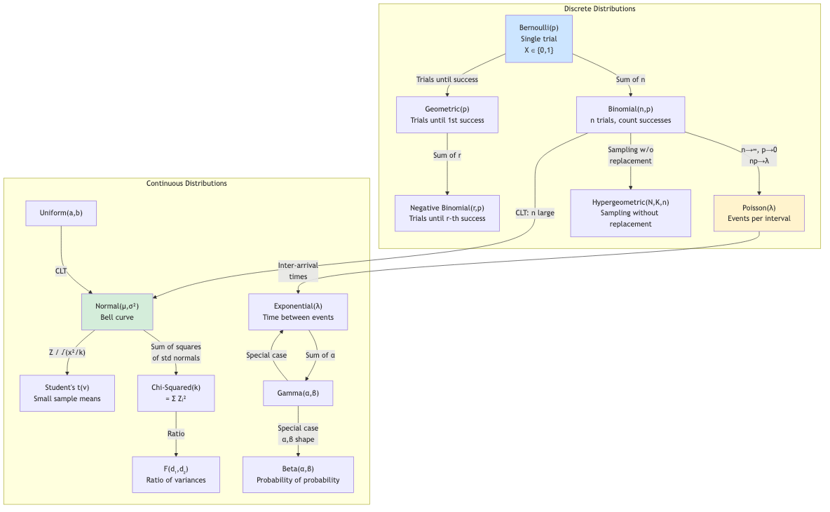
Relationships Between Distributions
Bernoulli(p) ← sum of n → Binomial(n, p)
                              ↓ n→∞, np→λ
                           Poisson(λ)
                              ↓ inter-arrival
                           Exponential(λ)
                              ↓ sum of α
                           Gamma(α, λ)
                              ↓ α=n/2, λ=1/2
                           Chi-squared(n)

Normal(μ,σ²) ← CLT ← sum of many iid

Z² ~ Chi-squared(1)
Z/√(χ²ₙ/n) ~ t(n)
(χ²ₘ/m)/(χ²ₙ/n) ~ F(m,n)
Applications in CS
- Queueing theory: Poisson arrivals, exponential service times → M/M/1 queue. Gamma for k-stage service.
- Machine learning: Gaussian noise models, Bernoulli for binary classification, Beta prior for A/B testing, Dirichlet for topic models.
- Bayesian inference: Beta-Binomial, Gamma-Poisson, Normal-Normal conjugate pairs enable closed-form posterior updates.
- Reliability engineering: Exponential/Weibull for failure times. Gamma for aggregate failure counts.
- Network modeling: Poisson process for packet arrivals. Exponential for inter-arrival times.
- Statistical testing: Chi-squared for goodness-of-fit and independence. t-distribution for means. F-distribution for ANOVA.
- Cryptography: Uniform distribution for key generation. Chi-squared for frequency analysis attacks.
- Simulation: Generating random variates from various distributions (inverse transform, Box-Muller for normal, acceptance-rejection).