Statistical Inference

Statistical inference draws conclusions about populations from sample data. It bridges the gap between observed data and general principles.

Point Estimation

A point estimator θ̂ is a single value used to estimate an unknown parameter θ.

Properties of Estimators

Bias: Bias(θ̂) = E[θ̂] - θ. An estimator is unbiased if E[θ̂] = θ.

• x̄ is unbiased for μ
• s² (with n-1 denominator) is unbiased for σ²
• s is biased for σ (but consistent)

Variance: Var(θ̂). Lower is better. The standard error SE(θ̂) = √Var(θ̂).

Mean Squared Error: MSE(θ̂) = Var(θ̂) + Bias²(θ̂). Combines bias and variance.

Consistency: θ̂ converges to θ as n → ∞ (in probability).

Efficiency: Among unbiased estimators, the one with smallest variance. The Cramér-Rao lower bound gives the minimum possible variance.

Maximum Likelihood Estimation (MLE)

Find θ that maximizes the likelihood function:

L(θ | x) = P(x | θ) = Πᵢ f(xᵢ | θ)

In practice, maximize the log-likelihood (easier, same maximum):

ℓ(θ) = Σᵢ ln f(xᵢ | θ)

Set ∂ℓ/∂θ = 0 and solve.

Example: Normal distribution MLE.

ℓ(μ, σ²) = -n/2 ln(2π) - n/2 ln(σ²) - Σ(xᵢ-μ)²/(2σ²)
∂ℓ/∂μ = 0 → μ̂ = x̄
∂ℓ/∂σ² = 0 → σ̂² = (1/n) Σ(xᵢ - x̄)²   (biased!)

Properties of MLE:

• Asymptotically unbiased, consistent, efficient
• Asymptotically normal: θ̂ → N(θ, I(θ)⁻¹) where I(θ) is the Fisher information
• Invariant: if θ̂ is MLE of θ, then g(θ̂) is MLE of g(θ)

Method of Moments (MOM)

Set sample moments equal to population moments and solve:

(1/n) Σ xᵢᵏ = E[Xᵏ]    for k = 1, 2, ...

Simpler than MLE but generally less efficient.

Maximum A Posteriori (MAP)

Bayesian point estimate. Maximize the posterior:

θ̂_MAP = argmax P(θ | x) = argmax P(x | θ) P(θ)

MLE with a prior P(θ). When prior is uniform, MAP = MLE.

Interval Estimation

Confidence Intervals

A (1-α) confidence interval [L, U] satisfies:

P(L ≤ θ ≤ U) = 1 - α

Interpretation: If we repeated the experiment many times and computed the CI each time, (1-α)×100% of the intervals would contain the true θ.

CI for Mean (σ known)

x̄ ± z_{α/2} · σ/√n

where z_{α/2} is the critical value from N(0,1). For 95% CI: z = 1.96.

CI for Mean (σ unknown)

Use the t-distribution with n-1 degrees of freedom:

x̄ ± t_{α/2, n-1} · s/√n

CI for Proportion

For large n:

p̂ ± z_{α/2} √(p̂(1-p̂)/n)

where p̂ = successes/n. Requires np̂ ≥ 5 and n(1-p̂) ≥ 5.

Factors Affecting CI Width

• Confidence level: Higher confidence → wider interval
• Sample size: Larger n → narrower interval (width ∝ 1/√n)
• Variability: Larger σ → wider interval

Sample Size Determination

For a desired margin of error E at confidence level 1-α:

n = (z_{α/2} · σ / E)²     (for means)
n = (z_{α/2})² · p(1-p) / E²  (for proportions, use p = 0.5 if unknown)

Hypothesis Testing

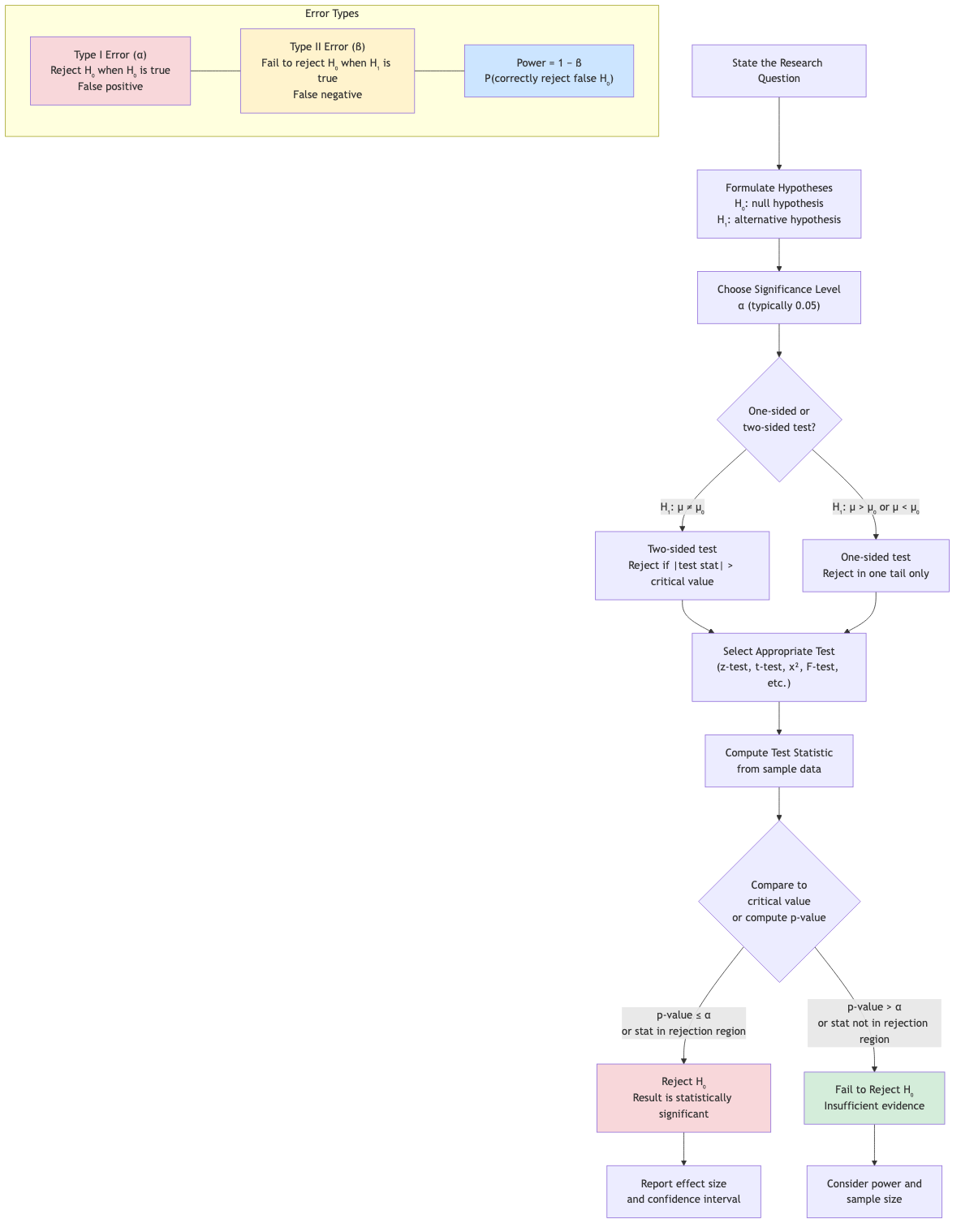
Framework

1. Null hypothesis H₀: The default/status quo claim (e.g., μ = μ₀).
2. Alternative hypothesis H₁: What we want to show (e.g., μ ≠ μ₀, μ > μ₀, or μ < μ₀).
3. Test statistic: A function of the sample data.
4. Decision rule: Reject H₀ if the test statistic falls in the rejection region.

Types of Errors

| | H₀ true | H₀ false | |---|---|---| | Reject H₀ | Type I error (α) | Correct (Power = 1-β) | | Fail to reject H₀ | Correct | Type II error (β) |

• α (significance level): P(Type I error) = P(reject H₀ | H₀ true). Typically 0.05.
• β: P(Type II error) = P(fail to reject H₀ | H₁ true).
• Power = 1 - β = P(reject H₀ | H₁ true). Higher is better.

p-Value

The p-value is the probability of observing a test statistic as extreme as (or more extreme than) the observed value, assuming H₀ is true.

• p ≤ α: Reject H₀ ("statistically significant")
• p > α: Fail to reject H₀

p-value is NOT the probability that H₀ is true.

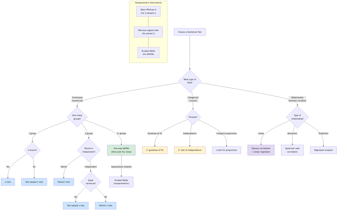
Common Tests

Z-test (σ known): z = (x̄ - μ₀) / (σ/√n).

t-test (σ unknown): t = (x̄ - μ₀) / (s/√n), df = n-1.

Two-sample t-test: t = (x̄₁ - x̄₂) / √(s₁²/n₁ + s₂²/n₂).

Paired t-test: t-test on the differences dᵢ = xᵢ - yᵢ.

Chi-squared test: For categorical data (goodness of fit, independence).

F-test: Comparing two variances, ANOVA.

One-Tailed vs Two-Tailed

• Two-tailed (H₁: μ ≠ μ₀): Reject if |test stat| > critical value.
• Right-tailed (H₁: μ > μ₀): Reject if test stat > critical value.
• Left-tailed (H₁: μ < μ₀): Reject if test stat < critical value.

Likelihood Ratio Tests

The likelihood ratio statistic:

Λ = L(θ̂₀) / L(θ̂)

where θ̂₀ is the MLE under H₀ and θ̂ is the unrestricted MLE.

Wilks' theorem: -2 ln(Λ) → χ²(k) as n → ∞, where k = difference in number of parameters.

This provides a general framework for comparing nested models.

Multiple Testing

Testing many hypotheses simultaneously inflates Type I error.

Bonferroni correction: Use α/m for each of m tests. Conservative.

Benjamini-Hochberg (FDR control): Sort p-values, reject pᵢ ≤ (i/m)·α. Controls false discovery rate.

Power Analysis

Power depends on:

• Effect size (larger effect → higher power)
• Sample size (larger n → higher power)
• Significance level (larger α → higher power)
• Variability (smaller σ → higher power)

Use power analysis to determine the sample size needed to detect a given effect size.

Cohen's conventions: Small effect d = 0.2, medium d = 0.5, large d = 0.8 (for two-group comparison, d = (μ₁-μ₂)/σ).

Applications in CS

• A/B testing: Compare conversion rates, latency, revenue between variants. Two-sample tests, confidence intervals for the difference.
• Performance benchmarking: Is system A faster than system B? Paired t-test on matched workloads.
• ML model evaluation: Is model A's accuracy significantly better than model B's? McNemar's test, bootstrap confidence intervals.
• Anomaly detection: Test if observed metrics deviate significantly from baseline. Control charts use CI principles.
• Database optimization: Test if a query plan change improves performance significantly.
• Clinical trials: Sequential testing, interim analyses, adaptive designs.
• Scientific computing: Validation of simulation results against analytical solutions.