Pipelining
Pipelining is the key technique for high-throughput instruction execution. Like an assembly line, multiple instructions are in different stages of execution simultaneously.
Pipeline Concept
The Laundry Analogy
Without pipelining: Wash → Dry → Fold → Store, then start next load. With pipelining: Start a new load every stage-time. All machines busy simultaneously.
Five-Stage Pipeline (Classic RISC)
Time →  1    2    3    4    5    6    7    8
I1:    IF   ID   EX   MEM  WB
I2:         IF   ID   EX   MEM  WB
I3:              IF   ID   EX   MEM  WB
I4:                   IF   ID   EX   MEM  WB
| Stage | Name | Activity |
|---|---|---|
| IF | Instruction Fetch | Read instruction from I-cache; PC ← PC + 4 |
| ID | Instruction Decode | Decode opcode; read registers; sign-extend immediate |
| EX | Execute | ALU operation; compute branch target; compute address |
| MEM | Memory Access | Read/write data cache (load/store only) |
| WB | Write Back | Write result to register file |
Pipeline Registers
Between each stage, pipeline registers store intermediate values:
IF/ID: Instruction, PC+4
ID/EX: Register values, immediate, control signals, PC+4
EX/MEM: ALU result, write data, control signals
MEM/WB: Memory data, ALU result, control signals
These registers are clocked — at each edge, all stages advance simultaneously.
Performance
Ideal speedup: S = number of stages (k). With k = 5, throughput is 5× a non-pipelined processor.
Actual speedup: Less than k due to:
- Pipeline register overhead (adds to clock period)
- Hazards causing stalls
- Unequal stage delays (clock limited by slowest stage)
Throughput: Ideally 1 instruction per cycle (CPI = 1).
Latency: Each individual instruction still takes k cycles. Pipelining improves throughput, not latency.
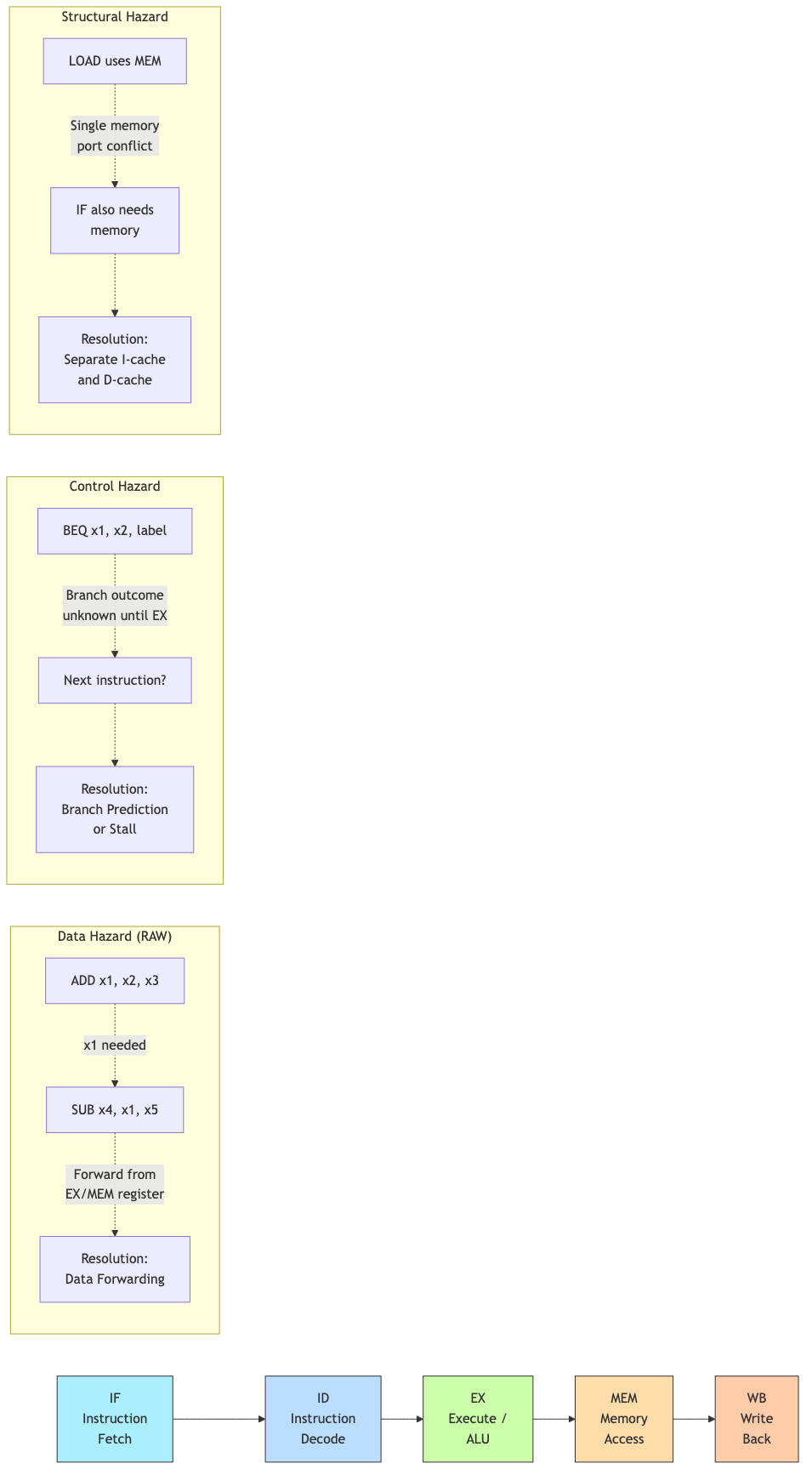
Pipeline Hazards
Situations that prevent the next instruction from executing in the next clock cycle.
Structural Hazards
Two instructions need the same hardware resource simultaneously.
Example: Single memory for both instructions and data. IF and MEM stages conflict.
Solution: Separate instruction and data caches (Harvard architecture). Modern processors always do this.
Example: Single-port register file — simultaneous read (ID) and write (WB).
Solution: Write in first half of cycle, read in second half. Or multi-port register file.
Data Hazards
An instruction depends on the result of a previous instruction still in the pipeline.
Types:
- RAW (Read After Write): Most common. Instruction reads a register before a prior instruction writes it.
- WAR (Write After Read): Later instruction writes before earlier reads. Occurs in out-of-order execution.
- WAW (Write After Write): Two instructions write the same register. Occurs in out-of-order execution.
Example (RAW):
ADD x1, x2, x3    // Writes x1 in WB (cycle 5)
SUB x4, x1, x5    // Reads x1 in ID (cycle 3) — x1 not yet written!
Forwarding (Bypassing)
Route the result directly from where it's produced to where it's needed, without waiting for the write-back stage.
EX/MEM forwarding: Result available after EX → forward to next instruction's EX input
MEM/WB forwarding: Result available after MEM → forward to instruction 2 stages later
Hardware: Multiplexers at ALU inputs. Forwarding unit detects hazards and selects the correct input source.
Time →  1    2    3    4    5
ADD:   IF   ID   EX   MEM  WB
SUB:        IF   ID   EX←──┘ (forward from EX/MEM)
                      ↑
                  ALU input comes from forward path, not register file
Load-Use Hazard
A load followed immediately by an instruction using the loaded value cannot be resolved by forwarding alone — the data isn't available until after the MEM stage.
LW  x1, 0(x2)    // Data available after MEM (cycle 4)
ADD x3, x1, x4   // Needs x1 in EX (cycle 3) — too early!
Solution: Insert a pipeline bubble (1-cycle stall). The hardware detects the load-use hazard and inserts a NOP.
Compiler optimization: Schedule an independent instruction between the load and its use ("load delay slot scheduling") to avoid the stall.
Control Hazards (Branch Hazards)
The pipeline doesn't know which instruction to fetch next until the branch is resolved.
Problem: Branch decision is made in EX (cycle 3). But we've already fetched 2 instructions that may be wrong (if branch taken).
BEQ x1, x2, target  // Branch decided in EX
IF   ID   EX ← branch decided here
     IF   ID  ← fetched speculatively
          IF  ← fetched speculatively (may be wrong)
Solutions
1. Stall (flush): Always stall until branch is resolved. 2-cycle penalty. Simple but slow.
2. Assume not taken: Always fetch the next sequential instruction. If branch is taken, flush the incorrect instructions (2-cycle penalty). If not taken, no penalty. Works well for loops (most backward branches are taken, most forward are not).
3. Delayed branch: The instruction after the branch (in the "delay slot") always executes regardless of branch outcome. Compiler fills the slot with a useful instruction. Used in MIPS. Considered a design mistake — complicates the ISA permanently.
4. Branch prediction: Predict the outcome and speculatively fetch along the predicted path. If wrong, flush and recover. See below.
Branch Prediction
Static Prediction
- Always not taken: Fetch PC + 4. Penalty on taken branches.
- Always taken: Fetch branch target. Penalty on not-taken branches.
- Backward taken, forward not taken (BTFNT): Backward branches are loops (usually taken). Forward branches are if-statements (often not taken). ~65% accuracy.
Dynamic Prediction
Use runtime history to predict future branches.
Branch History Table (BHT)
Index by low-order PC bits. Each entry stores a predictor.
1-bit predictor: Remember last outcome. Problem: always mispredicts twice on loop exit.
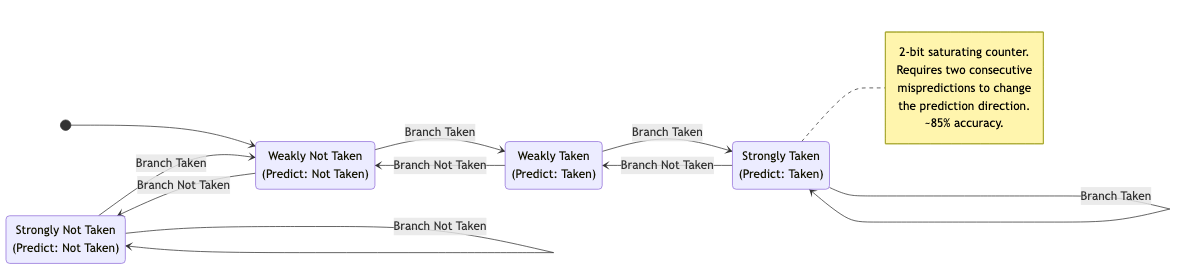
2-bit saturating counter: States: Strongly Not Taken (00), Weakly Not Taken (01), Weakly Taken (10), Strongly Taken (11). Takes two mispredictions to change prediction. ~85% accuracy.
       Taken           Taken
SNT(00) → WNT(01) → WT(10) → ST(11)
  ↑ Not Taken    ↑ Not Taken    ↑
  └──────────────┘              │
                   Not Taken    │
                   WT(10) ← ST(11)
Branch Target Buffer (BTB)
Caches the target address of recently taken branches. Indexed by PC. If the branch is predicted taken and the target is in the BTB, we can fetch from the target immediately (no delay for address computation).
Correlating Predictors
Use the outcome of recent branches to predict the current branch.
(m, n) predictor: Use the last m branch outcomes (global history) to select among 2ᵐ separate n-bit predictors per branch.
Example: (2, 2) predictor: 4 separate 2-bit counters per branch, selected by the last 2 branch outcomes. ~92% accuracy.
Tournament Predictors
Combine multiple predictors with a selector that learns which predictor works better for each branch.
Alpha 21264: Local (per-branch history) + global (correlating) + selector. ~95%+ accuracy.
Neural Branch Predictors
Use a perceptron (simple neural network) to predict branches. Each input is a past branch outcome. Weights learned online.
TAGE predictor: Tagged geometric history length predictor. Multiple tables indexed by different history lengths. State of the art. Used in modern Intel/AMD processors. >99% accuracy.
Misprediction Penalty
When a prediction is wrong:
- Flush incorrectly fetched/decoded instructions
- Restart fetch at the correct address
- Wasted cycles = pipeline depth to the branch resolution stage
Modern processors: 15-20 cycle misprediction penalty. This is why high accuracy matters enormously.
Pipeline Performance
CPI Breakdown
CPI = 1 + stall_cycles_per_instruction

CPI = 1 + (load_stalls × load_fraction) + (branch_penalty × branch_fraction × mispredict_rate)
Example: 20% loads with 50% load-use stalls (1 cycle each). 15% branches with 5% mispredict rate, 2-cycle penalty.
CPI = 1 + (0.2 × 0.5 × 1) + (0.15 × 0.05 × 2) = 1 + 0.10 + 0.015 = 1.115
Speedup
Speedup = CPI_unpipelined / CPI_pipelined × (Clock_pipelined / Clock_unpipelined)
Pipeline register overhead slightly increases clock period but dramatically improves throughput.
Deeper Pipelines
More stages → higher clock frequency but:
- More hazards (longer forwarding paths, higher branch penalty)
- More pipeline register overhead
- Diminishing returns
Historical trend: Pentium 4 had 31 stages (too deep — high misprediction penalty). Modern designs: 14-20 stages.
Applications in CS
- Compiler optimization: Instruction scheduling to avoid stalls. Loop unrolling to reduce branch overhead. Software pipelining for loops.
- Performance analysis: Understanding pipeline behavior helps interpret profiler data (IPC, branch misprediction rate, cache miss stalls).
- Operating systems: Context switch must save/restore pipeline state. Interrupt handling flushes the pipeline.
- Security: Spectre exploits speculative execution (branch prediction + cache side channel). Meltdown exploits out-of-order execution. Understanding the pipeline is essential for understanding these attacks.
- Embedded systems: Simpler pipelines (3-5 stages) for deterministic timing. WCET (worst-case execution time) analysis considers pipeline behavior.