Ray Tracing
Overview
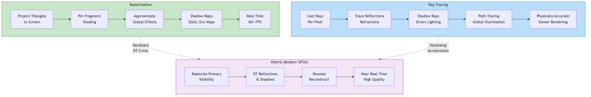
Ray tracing simulates the physics of light transport by tracing rays from the camera through each pixel into the scene. It naturally handles reflections, refractions, shadows, and global illumination, producing images of high physical accuracy at the cost of computational intensity.
Ray-Object Intersection
A ray is defined as: R(t) = O + t * D, where O is the origin, D is the direction, and t >= 0.
Ray-Sphere Intersection
Sphere: |P - C|^2 = r^2. Substituting the ray equation:
|O + tD - C|^2 = r^2
a*t^2 + b*t + c = 0

a = D . D
b = 2 * D . (O - C)
c = (O - C) . (O - C) - r^2

discriminant = b^2 - 4ac
t = (-b - sqrt(discriminant)) / (2a)    // nearest intersection
Ray-Triangle Intersection (Moller-Trumbore)
Compute barycentric coordinates directly:
E1 = V1 - V0,  E2 = V2 - V0,  T = O - V0
P = D x E2,  Q = T x E1

det = P . E1
t = (Q . E2) / det
u = (P . T) / det
v = (Q . D) / det

Hit if: t > 0, u >= 0, v >= 0, u + v <= 1
Requires only one division and avoids computing the triangle plane explicitly. Widely used in production ray tracers.
Ray-AABB Intersection (Slab Method)
For an axis-aligned bounding box with min/max corners:
for each axis i in {x, y, z}:
    t_min_i = (box_min_i - O_i) / D_i
    t_max_i = (box_max_i - O_i) / D_i
    if t_min_i > t_max_i: swap(t_min_i, t_max_i)

t_enter = max(t_min_x, t_min_y, t_min_z)
t_exit  = min(t_max_x, t_max_y, t_max_z)

Hit if: t_enter <= t_exit and t_exit >= 0
Critical for BVH traversal performance. Optimized implementations precompute 1/D and handle edge cases (D component = 0).
Bounding Volume Hierarchies (BVH)
Motivation
Naive ray tracing tests every ray against every primitive: O(N) per ray. BVH provides O(log N) average-case by organizing primitives into a hierarchy of bounding volumes.
BVH Structure
Binary tree where:
- Leaf nodes contain a small number of primitives (1-8)
- Internal nodes store an AABB encompassing all children
- Rays traverse the tree, skipping entire subtrees when the ray misses a node's AABB
Construction
Top-down (recursive partitioning):
- Compute AABB of all primitives
- Choose a split: partition primitives into two groups
- Recurse on each group until leaf criteria are met
Split heuristics:
- Midpoint: Split at the spatial midpoint of the longest axis
- Median: Split so each child has equal primitive count
- SAH (Surface Area Heuristic): Minimize expected traversal cost
Surface Area Heuristic (SAH)
The probability of a ray hitting a node is proportional to its surface area. SAH minimizes:
C(split) = C_traversal + (SA_left / SA_parent) * N_left * C_intersect
                        + (SA_right / SA_parent) * N_right * C_intersect
Evaluate across multiple candidate split positions (binning approach for efficiency: divide axis into K bins, compute cost for each partition).
BVH Traversal
stack = [root]
closest_hit = infinity

while stack is not empty:
    node = stack.pop()
    if not intersect_aabb(ray, node.aabb, closest_hit):
        continue
    if node.is_leaf:
        for each primitive in node:
            t = intersect(ray, primitive)
            if t < closest_hit:
                closest_hit = t
                hit_info = ...
    else:
        // Push far child first so near child is processed first
        if ray hits left child closer:
            stack.push(right), stack.push(left)
        else:
            stack.push(left), stack.push(right)
BVH Optimizations
- TLAS/BLAS (Vulkan RT): Two-level hierarchy. Bottom-level (BLAS) for individual meshes, top-level (TLAS) for instances with transforms. Allows instancing and animation without rebuilding the full BVH.
- BVH refitting: Update AABBs without restructuring the tree (for animated objects with small deformations).
- Compressed BVH: Quantize AABBs relative to parent to reduce memory.
Recursive Ray Tracing (Whitted-Style)
The classic algorithm (Whitted, 1980):
trace(ray, depth):
    hit = intersect_scene(ray)
    if no hit: return background_color

    color = ambient
    for each light:
        shadow_ray = ray from hit.point to light
        if not occluded(shadow_ray):
            color += shade(hit, light)      // diffuse + specular

    if hit.material.reflective and depth < max_depth:
        reflect_dir = reflect(ray.dir, hit.normal)
        color += hit.material.reflectance * trace(reflect_ray, depth + 1)

    if hit.material.transparent and depth < max_depth:
        refract_dir = refract(ray.dir, hit.normal, eta)
        color += hit.material.transmittance * trace(refract_ray, depth + 1)

    return color
Handles perfect mirrors and glass but not diffuse interreflection or soft effects.
Path Tracing
Monte Carlo Integration
Estimate the rendering equation integral by sampling random directions:
L_o(p, w_o) ~ (1/N) * sum_{i=1}^{N} f_r(w_i, w_o) * L_i(w_i) * cos(theta_i) / pdf(w_i)
Each sample traces a ray in direction w_i, recursively computing incoming radiance. Converges to the correct result as N -> infinity.
Path Tracing Algorithm
path_trace(ray, depth):
    hit = intersect_scene(ray)
    if no hit: return environment(ray.dir)
    if depth > max_depth: return 0 (or use Russian roulette)

    // Direct lighting (next event estimation)
    direct = 0
    sample light source: light_pos, light_pdf
    shadow_ray to light_pos
    if not occluded:
        direct = f_r * L_light * cos(theta) / light_pdf

    // Indirect lighting
    sample direction w_i from BRDF: brdf_pdf
    indirect = f_r * path_trace(new_ray, depth+1) * cos(theta) / brdf_pdf

    return emission + direct + indirect
Russian Roulette
Unbiased path termination: at each bounce, terminate with probability p. If continuing, scale the result by 1/(1-p):
if random() < p_terminate:
    return 0
result = trace_next_bounce() / (1 - p_terminate)
Commonly set p_terminate based on throughput (terminate low-energy paths more aggressively).
Importance Sampling
Sample directions proportional to the integrand to reduce variance.
- Cosine-weighted hemisphere: Sample proportional to cos(theta) for diffuse BRDFs. PDF = cos(theta)/pi.
- GGX importance sampling: Sample the half-vector from the NDF distribution. Generates directions where the BRDF is large.
- Light sampling: Sample points on light sources directly.
Multiple Importance Sampling (MIS)
Combine BRDF sampling and light sampling using the balance heuristic:
w_brdf = pdf_brdf^2 / (pdf_brdf^2 + pdf_light^2)
w_light = pdf_light^2 / (pdf_brdf^2 + pdf_light^2)

L = w_brdf * (f * L_i * cos / pdf_brdf) + w_light * (f * L_i * cos / pdf_light)
Reduces variance in all cases: when lights are small (light sampling wins) and when the BRDF is sharp (BRDF sampling wins).
Bidirectional Path Tracing
Trace paths from both the camera and light sources. Connect path vertices to form complete light paths. Handles caustics and difficult light transport paths that unidirectional path tracing struggles with (e.g., light through a small opening).
Photon Mapping (Jensen, 1996)
Two-pass algorithm:
- Photon tracing: Emit photons from lights, trace through the scene, store hits in a photon map (kd-tree)
- Rendering: Trace camera rays, estimate radiance at hit points by gathering nearby photons
L(p) ~ (1 / (pi * r^2)) * sum_{i in nearby photons} f_r * phi_i / N_emitted
Excels at caustics (focused light through glass). Progressive photon mapping removes bias by reducing the gather radius over iterations.
ReSTIR (Reservoir-based Spatio-Temporal Importance Resampling)
Efficient light sampling for scenes with millions of lights.
Core idea: Use reservoir sampling (Weighted Reservoir Sampling) to select high-contribution lights from a large pool using only a constant amount of memory per pixel.
1. Generate M candidate light samples per pixel
2. Use reservoir sampling to keep 1 sample proportional to its contribution
3. Temporal reuse: combine with previous frame's reservoir
4. Spatial reuse: combine with neighboring pixels' reservoirs
5. Shade using the selected light sample
Produces low-variance direct lighting with thousands of lights at near-interactive rates. ReSTIR GI extends this to indirect lighting.
Hardware Ray Tracing
RT Cores (NVIDIA RTX, AMD RDNA 3+, Intel Arc)
Dedicated hardware units that accelerate:
- BVH traversal: Fixed-function tree traversal of the acceleration structure
- Ray-triangle intersection: Parallel intersection testing
API Integration
Vulkan Ray Tracing:
- Build acceleration structures (TLAS/BLAS) with
vkBuildAccelerationStructuresKHR - Trace rays with
vkCmdTraceRaysKHR - Shader stages: Ray Generation, Closest Hit, Any Hit, Miss, Intersection, Callable
DXR (DirectX Raytracing):
DispatchRays()launches ray generation shaders- Shader table maps geometry to hit group shaders
Hybrid Rendering
Combine rasterization (primary visibility) with ray tracing (reflections, shadows, GI):
1. Rasterize G-Buffer (fast primary visibility)
2. Trace shadow rays from G-Buffer positions (RT shadows)
3. Trace reflection rays for glossy surfaces (RT reflections)
4. Denoise the noisy 1-spp results
Denoising is critical: temporal accumulation, spatial filters (A-SVGF, NVIDIA NRD), or neural denoisers reconstruct clean images from sparse ray-traced samples.