Control Fundamentals
Open-Loop vs Closed-Loop Control
Open-loop control applies a predetermined input without measuring the output. The controller has no knowledge of disturbances or plant variations.
Closed-loop (feedback) control measures the output, computes an error signal, and adjusts the input accordingly.
| Property | Open-Loop | Closed-Loop |
|---|---|---|
| Disturbance rejection | Poor | Good |
| Sensitivity to plant variation | High | Low |
| Stability risk | Low | Can be unstable |
| Complexity | Simple | Higher |
Feedback Principles
The fundamental feedback equation for a single-loop system with forward path G(s) and feedback path H(s):
Closed-loop TF: T(s) = G(s) / (1 + G(s)H(s))
For unity feedback (H(s) = 1):
T(s) = G(s) / (1 + G(s))
The error transfer function:
E(s)/R(s) = 1 / (1 + G(s)H(s))
Key insight: feedback reduces sensitivity to plant variations by the factor 1 + G(s)H(s), called the return difference.
Block Diagram Algebra
Standard block diagram operations:
Series (cascade):
G_total(s) = G1(s) * G2(s)
Parallel:
G_total(s) = G1(s) + G2(s)
Feedback loop:
G_total(s) = G(s) / (1 ± G(s)H(s))
Negative feedback uses +, positive feedback uses -.
Block diagram reduction rules:
- Moving a summing junction ahead of a block: insert the block's inverse in the moved path
- Moving a pickoff point ahead of a block: insert the block in the moved path
- Moving a summing junction past a block: insert the block in the moved path
- Moving a pickoff point past a block: insert the block's inverse in the moved path
Transfer Functions
A transfer function relates the Laplace transform of the output to the input, assuming zero initial conditions:
G(s) = Y(s)/U(s) = (b_m*s^m + ... + b_1*s + b_0) / (a_n*s^n + ... + a_1*s + a_0)
Poles: roots of the denominator -- determine stability and transient behavior. Zeros: roots of the numerator -- affect the shape of the transient response.
A system is proper if m <= n and strictly proper if m < n. Physical systems are always proper.
Factored form:
G(s) = K * (s - z_1)(s - z_2)...(s - z_m) / ((s - p_1)(s - p_2)...(s - p_n))
Partial fraction expansion decomposes G(s) for inverse Laplace transform computation.
Signal-Flow Graphs (Mason's Gain Formula)
An alternative to block diagrams using nodes (signals) and directed branches (gains).
Mason's gain formula:
T = (1/Delta) * sum_k(T_k * Delta_k)
Where:
T_k= gain of the k-th forward pathDelta= 1 - (sum of all loop gains) + (sum of products of non-touching loop pairs) - ...Delta_k= cofactor of Delta for path k (Delta evaluated with loops touching path k removed)
Example: For a system with two forward paths T1, T2 and three loops L1, L2, L3 where L1 and L2 don't touch:
Delta = 1 - (L1 + L2 + L3) + (L1*L2)
System Classification
Linearity
- Linear: superposition holds --
f(a*x1 + b*x2) = a*f(x1) + b*f(x2) - Nonlinear: saturation, dead zones, backlash, friction, hysteresis
Number of Inputs/Outputs
- SISO: Single-Input Single-Output -- classical control focus
- MIMO: Multiple-Input Multiple-Output -- requires matrix transfer functions
G(s)whereY(s) = G(s)U(s)
Time Variance
- Time-invariant (LTI): system parameters do not change with time
- Time-varying (LTV): parameters are functions of time, e.g., a spacecraft losing mass
Domain
- Continuous-time: described by differential equations, uses Laplace transform (s-domain)
- Discrete-time: described by difference equations, uses Z-transform (z-domain)
- Hybrid: mix of continuous and discrete subsystems (sampled-data systems)
Causality and Memory
- Causal: output depends only on current and past inputs
- Memoryless: output depends only on current input
- Dynamic: output depends on past inputs (has memory/state)
System Type and Error Constants
The system type is the number of pure integrators (poles at s = 0) in the open-loop transfer function.
For unity feedback with open-loop G(s):
| Input | Type 0 | Type 1 | Type 2 |
|---|---|---|---|
| Step (1/s) | e_ss = 1/(1+Kp) | 0 | 0 |
| Ramp (1/s^2) | infinity | 1/Kv | 0 |
| Parabola (1/s^3) | infinity | infinity | 1/Ka |
Error constants:
Kp = lim(s->0) G(s)           (position constant)
Kv = lim(s->0) s*G(s)         (velocity constant)
Ka = lim(s->0) s^2*G(s)       (acceleration constant)
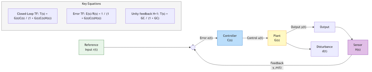
Typical Feedback Control Architecture
R(s) -->(+)--> C(s) --> G_plant(s) --> Y(s)
         ^(-)                           |
         |--- H(s) <-------------------|
Components:
- R(s): reference input (setpoint)
- E(s) = R(s) - H(s)Y(s): error signal
- C(s): controller (compensator)
- G_plant(s): plant (process to be controlled)
- H(s): sensor/feedback element
- D(s): disturbance (enters at various points)
Disturbance rejection transfer function (disturbance at plant input):
Y(s)/D(s) = G_plant(s) / (1 + C(s)*G_plant(s)*H(s))
High controller gain reduces disturbance effect but risks instability.