Controller Design
PID Control
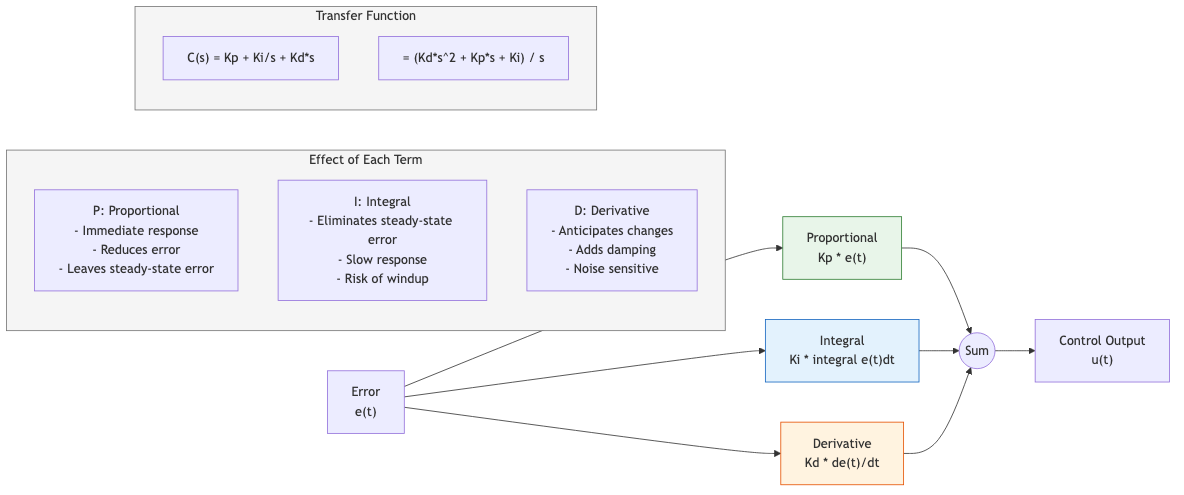
The most widely used controller in industry. Combines three terms:
u(t) = Kp*e(t) + Ki*integral(e(t)dt) + Kd*de(t)/dt
Transfer function:
C(s) = Kp + Ki/s + Kd*s = (Kd*s^2 + Kp*s + Ki) / s
| Term | Effect | Benefit | Risk |
|---|---|---|---|
| P (proportional) | Instantaneous correction | Reduces error | Steady-state error (alone) |
| I (integral) | Accumulates past error | Eliminates steady-state error | Oscillation, windup |
| D (derivative) | Anticipates future error | Improves transient, adds damping | Noise amplification |
Practical PID Implementation
Derivative filter: pure derivative is impractical; use Kd*s / (1 + tau_f*s) with tau_f = Kd/(N*Kp), N ~ 8-20.
Anti-windup: prevent integral term from growing during actuator saturation. Methods:
- Conditional integration: stop integrating when actuator saturates
- Back-calculation: feed back the difference between commanded and actual actuator output
Setpoint weighting: apply P and D to output only (not error) to reduce overshoot on setpoint changes while maintaining disturbance rejection.
Ziegler-Nichols Tuning
Method 1 -- Step response (open-loop): Apply step input, measure the S-shaped response. Identify delay L and time constant T from the tangent line at the inflection point.
| Controller | Kp | Ti | Td |
|---|---|---|---|
| P | T/L | - | - |
| PI | 0.9*T/L | L/0.3 | - |
| PID | 1.2*T/L | 2*L | 0.5*L |
Method 2 -- Ultimate gain (closed-loop): Increase proportional gain until sustained oscillation. Record ultimate gain K_u and period P_u.
| Controller | Kp | Ti | Td |
|---|---|---|---|
| P | 0.5*Ku | - | - |
| PI | 0.45*Ku | Pu/1.2 | - |
| PID | 0.6*Ku | Pu/2 | Pu/8 |
Ziegler-Nichols gives aggressive tuning (quarter-decay ratio, ~25% overshoot). Often needs detuning.
Auto-Tuning (Relay Feedback)
Replace the controller with a relay. The system oscillates at approximately the ultimate frequency. Measure K_u and P_u from the relay oscillation, then apply tuning rules. Avoids the need to manually find the stability boundary.
Lead and Lag Compensators
Lead Compensator
C(s) = Kc * (s + z) / (s + p) where p > z (p = z/alpha, 0 < alpha < 1)
Adds phase lead near crossover frequency. Equivalent to PD control with a high-frequency pole.
Design procedure:
- Set Kc for steady-state error requirement
- Compute required phase lead:
phi_max = PM_desired - PM_current + margin - Calculate alpha:
sin(phi_max) = (1 - alpha) / (1 + alpha) - Place maximum phase at new gain crossover:
omega_max = 1 / (T*sqrt(alpha)) - Compute
T = 1 / (omega_max * sqrt(alpha)), thenz = 1/T,p = 1/(alpha*T)
Lag Compensator
C(s) = Kc * (s + z) / (s + p) where z > p (acts at low frequencies)
Increases low-frequency gain without significantly affecting phase near crossover. Equivalent to PI control approximation.
Design procedure:
- Set gain for desired PM at a chosen crossover frequency
- Place zero z at 1/10th of crossover
- Place pole p to achieve required low-frequency gain boost:
p = z * (current_gain / desired_gain)
Lead-Lag Compensator
Combines both: lag for steady-state accuracy, lead for transient response/stability margins. Design each part separately (lag first, then lead at higher frequencies).
State Feedback (Pole Placement)
Given controllable system x' = Ax + Bu, apply control law:
u = -K*x + r
Closed-loop: x' = (A - B*K)*x + B*r
Choose K to place eigenvalues of (A - B*K) at desired locations.
Ackermann's Formula (SISO)
K = [0, 0, ..., 1] * C_ctrl^(-1) * phi_d(A)
Where C_ctrl = [B, AB, ..., A^(n-1)B] and phi_d(A) = A^n + alpha_{n-1}*A^{n-1} + ... + alpha_0*I is the desired characteristic polynomial evaluated at A.
Design Considerations
- Only eigenvalues can be assigned, not eigenvectors (for SISO)
- Requires full state measurement (use observer if not available)
- Moving poles far left requires large control effort
- Cannot move transmission zeros
Observer Design (State Estimation)
When states are not directly measurable, estimate them:
x_hat' = A*x_hat + B*u + L*(y - C*x_hat)
Error dynamics: e' = (A - L*C)*e where e = x - x_hat.
Choose L to place eigenvalues of (A - L*C) -- requires observability.
Dual of pole placement: observer design for (A, C) is equivalent to state feedback for (A^T, C^T).
Separation Principle
The controller gain K and observer gain L can be designed independently. The combined system has eigenvalues equal to the union of the state feedback and observer eigenvalues.
Rule of thumb: make observer poles 2-5x faster than controller poles.
Linear Quadratic Regulator (LQR)
Find u = -K*x minimizing the cost:
J = integral_0^inf (x^T*Q*x + u^T*R*u) dt
Where Q >= 0 (state penalty) and R > 0 (control penalty).
Solution: K = R^(-1) * B^T * P where P is the unique positive-definite solution of the algebraic Riccati equation (ARE):
A^T*P + P*A - P*B*R^(-1)*B^T*P + Q = 0
LQR Properties
- Guaranteed stability (if controllable)
- Guaranteed gain margin >= 6 dB and phase margin >= 60 deg (SISO)
- Robustness degrades for MIMO systems
- Tuning: increase Q/R ratio for faster response (more control effort)
- Bryson's rule:
Q_ii = 1/(max x_i)^2,R_jj = 1/(max u_j)^2
Linear Quadratic Gaussian (LQG)
Combines LQR with Kalman filter (optimal observer for systems with Gaussian noise):
x' = A*x + B*u + G*w     (process noise w ~ N(0, W))
y  = C*x + v             (measurement noise v ~ N(0, V))
Kalman filter gain:
L = P_e * C^T * V^(-1)
Where P_e solves the dual ARE: A*P_e + P_e*A^T - P_e*C^T*V^(-1)*C*P_e + G*W*G^T = 0.
LQG = LQR gain + Kalman filter, applying separation principle.
Warning: LQG does NOT inherit LQR's gain/phase margin guarantees. Robustness must be verified separately, motivating robust control methods (H-infinity, etc.).
Integral Action in State Feedback
To eliminate steady-state error, augment the state with integral of the error:
x_I' = r - C*x
u = -K*x - K_I*x_I
Augmented system: design K and K_I jointly via pole placement or LQR on the extended system.