Hash Tables

Hash tables provide average O(1) lookup, insert, and delete by mapping keys to array indices via a hash function. They are the most widely used data structure in software engineering.

Hash Functions

A hash function h maps keys to integers (bucket indices):

h: Key → {0, 1, ..., m-1}

Properties of Good Hash Functions

1. Deterministic: Same key always produces the same hash.
2. Uniform distribution: Keys spread evenly across buckets.
3. Fast to compute: O(key_length).
4. Avalanche effect: Small change in key → large change in hash.

Common Hash Functions

Division method: h(k) = k mod m. Choose m as a prime not close to a power of 2.

Multiplication method: h(k) = ⌊m × (k × A mod 1)⌋ where A ≈ (√5 - 1)/2 ≈ 0.6180. Works well for any m.

For strings (polynomial rolling hash):

h(s) = (s[0] × pⁿ⁻¹ + s[1] × pⁿ⁻² + ... + s[n-1]) mod m

where p is a prime (31 or 37 commonly). Compute efficiently with Horner's method.

FNV-1a: Fast non-cryptographic hash. Used in many hash tables.

SipHash: Pseudorandom function designed for hash tables. Resistant to hash-flooding DoS attacks. Default in Rust's HashMap.

xxHash, wyhash: Very fast non-cryptographic hashes. Used in high-performance applications.

Universal Hashing

A family of hash functions H is universal if for any two distinct keys x ≠ y:

P_{h∈H}[h(x) = h(y)] ≤ 1/m

Choose h randomly from H at initialization. Guarantees O(1) expected performance regardless of key distribution.

Carter-Wegman family: h(k) = ((ak + b) mod p) mod m, where a, b are random, p is prime.

Perfect Hashing

A hash function with no collisions for a known set of keys.

Static perfect hashing: Construct a two-level hash table. First level: universal hashing into m buckets. Second level: perfect hash for each bucket (using m_i² slots for m_i elements in bucket i). Total space: O(n).

Minimal perfect hashing: Maps n keys to exactly {0, 1, ..., n-1} with no collisions. Used in compilers, databases, and read-only dictionaries.

Consistent Hashing

Maps both keys and nodes to a circular hash space (ring). Each key is assigned to the next node clockwise on the ring.

Adding/removing a node only affects keys near that position on the ring — O(K/N) keys remapped on average (vs O(K) for regular hashing).

Virtual nodes: Each physical node maps to multiple positions on the ring, improving balance.

Used in: Distributed caches (Memcached), CDNs, distributed databases (Cassandra, DynamoDB), load balancers.

Collision Resolution

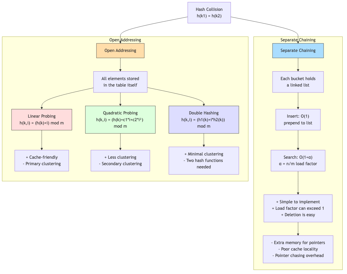
Separate Chaining

Each bucket stores a linked list (or other collection) of entries.

Bucket 0: → (key_a, val_a) → (key_b, val_b)
Bucket 1: → (key_c, val_c)
Bucket 2: (empty)
Bucket 3: → (key_d, val_d) → (key_e, val_e) → (key_f, val_f)

Load factor α = n/m (elements / buckets).

Expected chain length: α (with uniform hashing). Search time: O(1 + α). Advantage: Simple. Works well for high load factors. Disadvantage: Pointer overhead. Cache-unfriendly (linked list traversal).

Optimization: Java's HashMap switches from linked list to red-black tree when a bucket has > 8 entries.

Open Addressing

All entries stored in the table itself. On collision, probe for an empty slot.

Load factor must be < 1 (typically ≤ 0.7-0.8).

Linear Probing

Probe sequence: h(k), h(k)+1, h(k)+2, ... (mod m).

Insert key with h(k) = 3:
Table: [_][_][_][X][X][_][_]  ← slots 3,4 occupied
Probe: 3(X), 4(X), 5(empty) → insert at 5

Primary clustering: Long runs of occupied slots form, slowing search. Expected probe length: 1/(1-α)² for unsuccessful search.

Despite clustering, linear probing is often the fastest in practice due to excellent cache locality (probes hit the same cache line).

Quadratic Probing

Probe sequence: h(k), h(k)+1², h(k)+2², h(k)+3², ...

Reduces primary clustering but can cause secondary clustering (keys with the same hash follow the same probe sequence).

Issue: May not visit all slots. Guaranteed to find an empty slot if m is prime and α < 0.5.

Double Hashing

Probe sequence: h₁(k), h₁(k) + h₂(k), h₁(k) + 2×h₂(k), ...

Two independent hash functions. Eliminates both primary and secondary clustering.

h₂(k) must never be 0 and must be coprime to m (e.g., h₂(k) = 1 + k mod (m-1) with m prime).

Robin Hood Hashing

On insertion, if the new key has traveled fewer probes than the current occupant, swap them (the "richer" gives way to the "poorer").

Effect: Reduces variance of probe lengths. Maximum probe length is O(log n) with high probability.

Advantage: More predictable performance. Deletion is simpler than standard open addressing.

Cuckoo Hashing

Use two hash functions h₁, h₂. Each key is in exactly one of two positions.

Insert: Place in h₁(k). If occupied, kick out the existing key and place it at its alternative position. Repeat (may cascade). If a cycle is detected, rehash with new functions.

Lookup: Check exactly 2 positions. Worst-case O(1) lookup!

Load factor: Must be < 50% (two tables) or use more hash functions (d-ary cuckoo allows higher load).

Load Factor and Rehashing

When load factor exceeds a threshold (typically 0.75 for chaining, 0.7 for open addressing):

1. Allocate a new table (typically 2× size).
2. Reinsert all entries with the new hash function.
3. Free the old table.

Cost: O(n) for rehashing. Amortized O(1) per operation (similar to dynamic array).

Probabilistic Data Structures

Bloom Filter

A space-efficient probabilistic set membership test.

Structure: Bit array of m bits, k hash functions.

Insert: Set bits h₁(x), h₂(x), ..., hₖ(x) to 1.

Query: Check all k bits. If all are 1 → "probably in set." If any is 0 → "definitely not in set."

False positive rate: (1 - e^(-kn/m))^k. Optimal k = (m/n) × ln 2.

No false negatives. Cannot delete elements (use counting Bloom filter instead).

Space: ~10 bits per element for 1% false positive rate. Much smaller than storing actual elements.

Used in: Database query optimization (skip non-existent keys), network routing, spell checkers, CDN caching, distributed systems (avoid unnecessary network requests).

Count-Min Sketch

Estimates frequency of elements in a data stream.

Structure: d × w table of counters, d hash functions.

Insert(x): Increment counters at h₁(x), h₂(x), ..., hₐ(x).

Query(x): Return min(counter[h₁(x)], ..., counter[hₐ(x)]).

Error: Overestimates by at most ε×n with probability 1-δ, where w = ⌈e/ε⌉ and d = ⌈ln(1/δ)⌉.

Used in: Network traffic analysis, database query optimization, trending topics.

HyperLogLog

Estimates the number of distinct elements in a data stream.

Uses the observation: if you hash elements uniformly, the maximum number of leading zeros in any hash ≈ log₂(n).

Space: ~12 KB for counting up to 10⁹ distinct elements with ~2% error.

Used in: Redis (PFCOUNT), database cardinality estimation, web analytics (unique visitors).

Hash Table in Practice

Rust's HashMap

Uses SipHash by default (resistant to HashDoS). Robin Hood hashing with linear probing. Load factor threshold: 7/8.

map ← new HASH_MAP
INSERT(map, "key", 42)
val ← GET(map, "key")
IF val exists THEN
    PRINT val

Performance Considerations

• Hash function quality: Poor hash → many collisions → O(n) degradation.
• Cache performance: Open addressing (especially linear probing) is cache-friendly. Chaining is cache-hostile.
• Key size: Large keys → expensive hash computation. Consider pre-computing hashes.
• Load factor: Lower → faster but more memory. Higher → slower but less memory.

Applications in CS

• Databases: Hash indexes, hash joins, hash-based aggregation. Hash partitioning for distributed tables.
• Caching: In-memory caches (Redis, Memcached). LRU cache = hash map + doubly linked list.
• Compilers: Symbol tables, string interning, constant pools.
• Networking: Connection tracking (hash by 5-tuple), routing tables, NAT tables.
• Deduplication: File/block deduplication using content hashing.
• Distributed systems: Consistent hashing for load balancing, DHTs (Chord, Kademlia).
• Security: Password storage (hash + salt). Hash-based message authentication (HMAC).
• Version control: Git uses SHA-1 hashes for content-addressable storage.