Graph Coloring

Graph coloring assigns labels ("colors") to graph elements subject to constraints. It models resource allocation, scheduling, and conflict resolution.

Vertex Coloring

A proper vertex coloring of a graph G assigns a color to each vertex such that no two adjacent vertices share the same color.

A k-coloring uses at most k colors. A graph is k-colorable if a proper k-coloring exists.

Chromatic Number χ(G)

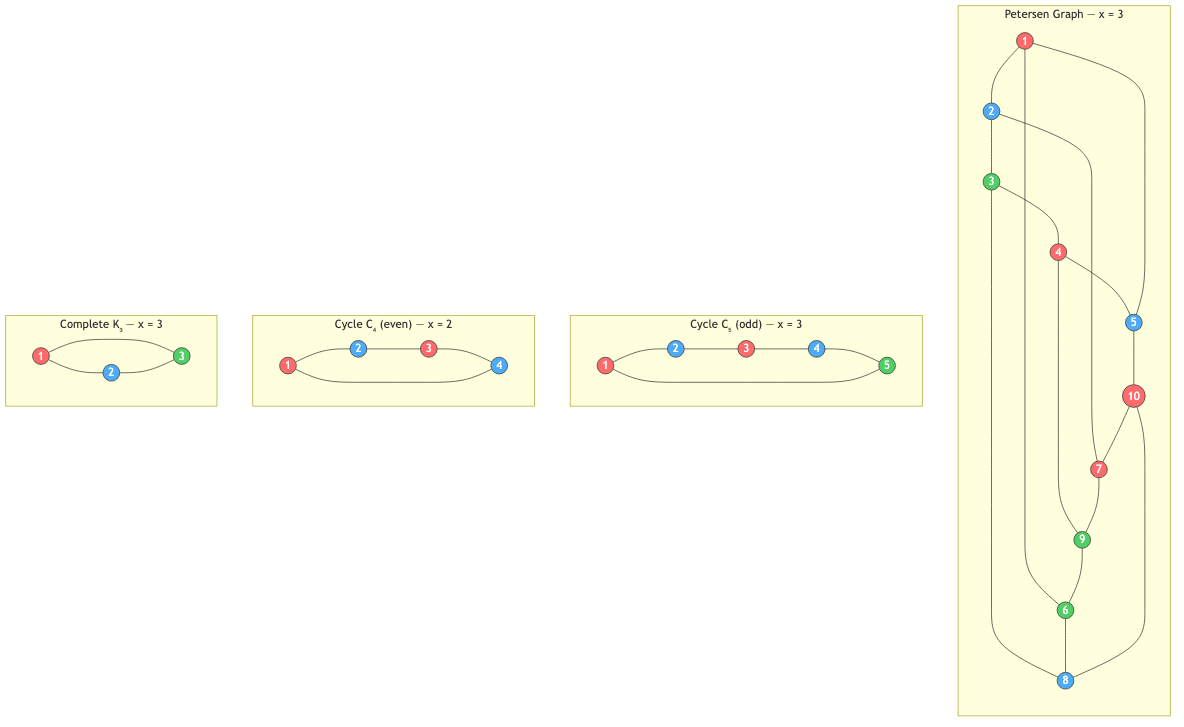
The chromatic number χ(G) is the minimum number of colors needed for a proper vertex coloring.

χ(G) = min{k | G is k-colorable}

Examples:

• χ(Kₙ) = n (complete graph — all vertices are adjacent)
• χ(empty graph) = 1 (no edges — 1 color suffices)
• χ(Cₙ) = 2 if n is even, 3 if n is odd
• χ(tree) = 1 if one vertex, 2 otherwise
• χ(bipartite graph) ≤ 2

Lower bounds on χ(G):

• χ(G) ≥ ω(G), where ω(G) is the clique number (size of largest complete subgraph).
• χ(G) ≥ n / α(G), where α(G) is the independence number (size of largest independent set).

Upper bounds:

• χ(G) ≤ Δ(G) + 1, where Δ(G) is the maximum degree (trivially, by greedy coloring).

Chromatic Polynomial

The chromatic polynomial P(G, k) counts the number of proper k-colorings of G.

Examples:

• P(Kₙ, k) = k(k-1)(k-2)...(k-n+1) = k^{(n)} (falling factorial)
• P(tree with n vertices, k) = k(k-1)ⁿ⁻¹
• P(Cₙ, k) = (k-1)ⁿ + (-1)ⁿ(k-1)

Deletion-contraction:

P(G, k) = P(G - e, k) - P(G / e, k)

where G - e is G with edge e removed, and G / e is G with edge e contracted.

Properties:

• P(G, k) is always a polynomial in k.
• The degree equals |V|.
• The leading coefficient is 1.
• χ(G) is the smallest positive integer k where P(G, k) > 0.

Edge Coloring

A proper edge coloring assigns colors to edges such that no two edges sharing an endpoint have the same color.

The chromatic index χ'(G) is the minimum number of colors needed.

Vizing's Theorem

For any simple graph G:

Δ(G) ≤ χ'(G) ≤ Δ(G) + 1

Graphs where χ'(G) = Δ(G) are Class 1. Graphs where χ'(G) = Δ(G) + 1 are Class 2.

Examples:

• Kₙ with n even: Class 1 (χ' = n - 1 = Δ)
• Kₙ with n odd: Class 2 (χ' = n = Δ + 1)
• Bipartite graphs: Always Class 1 (König's theorem: χ' = Δ)
• Petersen graph: Class 2 (Δ = 3, χ' = 4)

Determining whether a graph is Class 1 or Class 2 is NP-complete.

Four Color Theorem

Theorem (Appel & Haken, 1976): Every planar graph is 4-colorable.

χ(G) ≤ 4    for every planar graph G

This was the first major theorem proved with computer assistance (checking ~1,500 configurations). A simplified proof by Robertson et al. (1997) reduced to ~633 configurations. A fully formal proof was later verified in Coq.

Five Color Theorem: Easier to prove. Uses the fact that every planar graph has a vertex of degree ≤ 5 (by Euler's formula).

History: Conjectured by Guthrie (1852). False proofs by Kempe (1879, whose idea of "Kempe chains" is still useful) and Tait (1880). Correct proof in 1976.

Brooks' Theorem

For any connected graph G that is neither a complete graph nor an odd cycle:

χ(G) ≤ Δ(G)

(One less than the trivial bound of Δ + 1.)

Example: A 3-regular graph (not K₄, not odd cycle) is 3-colorable.

Greedy Coloring

Algorithm:

1. Order the vertices v₁, v₂, ..., vₙ.
2. For each vertex (in order), assign the smallest color not used by its already-colored neighbors.

Properties:

• Always produces a proper coloring.
• Uses at most Δ(G) + 1 colors (regardless of ordering).
• The number of colors used depends heavily on the vertex ordering.
• Optimal ordering gives χ(G) colors, but finding the optimal ordering is NP-hard.

Degeneracy ordering: Process vertices in reverse order of a sequence where each vertex has minimum degree in the remaining graph. This ordering guarantees at most d + 1 colors, where d is the degeneracy (maximum over all subgraphs H of the minimum degree of H).

Interval Graph Coloring

An interval graph has a vertex for each interval and edges between overlapping intervals.

Property: Interval graphs are perfect — χ(G) = ω(G) for the graph and all its induced subgraphs.

For interval graphs, the chromatic number equals the maximum number of mutually overlapping intervals (the clique number), and an optimal coloring can be found greedily by scanning left to right.

Application: Scheduling — intervals are tasks with start/end times, and colors are resources (rooms, machines, CPUs).

Map Coloring and Planar Graphs

Map coloring is equivalent to vertex coloring the dual graph. Each region becomes a vertex, and adjacent regions (sharing a border) become adjacent vertices.

The Four Color Theorem guarantees that any map can be colored with 4 colors.

Coloring and Independence

An independent set is a set of vertices with no edges between them. The independence number α(G) is the size of the largest independent set.

A k-coloring partitions V into k independent sets (color classes).

χ(G) · α(G) ≥ n
χ(G) ≥ n / α(G)

Complement relationship: χ(G) · α(G̅) ≥ n.

Perfect Graphs

A graph G is perfect if χ(H) = ω(H) for every induced subgraph H of G.

Strong Perfect Graph Theorem (Chudnovsky et al., 2006): A graph is perfect iff it contains no odd hole (odd cycle of length ≥ 5) and no odd antihole (complement of an odd cycle of length ≥ 5) as an induced subgraph.

Examples of perfect graph families:

• Bipartite graphs
• Interval graphs
• Chordal graphs (every cycle of length ≥ 4 has a chord)
• Comparability graphs
• Complements of perfect graphs (Perfect Graph Theorem, Lovász 1972)

Fractional and List Coloring

List Coloring

Each vertex v has a list L(v) of available colors. A list coloring assigns to each vertex a color from its list.

The list chromatic number (choosability) ch(G) is the smallest k such that G is L-colorable for every assignment of lists of size k.

Always: ch(G) ≥ χ(G). Can be strictly greater.

Fractional Coloring

A relaxation of coloring using linear programming. The fractional chromatic number χ_f(G) satisfies:

ω(G) ≤ χ_f(G) ≤ χ(G)

NP-Hardness

Determining χ(G) is NP-hard. Even deciding if χ(G) ≤ 3 is NP-complete.

k = 2: Polynomial (bipartiteness test via BFS/DFS). k = 3: NP-complete. k ≥ 3: NP-complete.

Approximation: No polynomial-time algorithm can approximate χ(G) within a factor of n^(1-ε) for any ε > 0, unless P = NP.

Real-World Applications

• Register allocation: Variables are vertices, conflicts are edges. Colors are CPU registers. Minimize registers = minimize colors. This is graph coloring on the interference graph.
• Scheduling: Time slots are colors. Conflicting events (same room/professor/student) are edges. Chromatic number = minimum time slots.
• Frequency assignment: Radio stations are vertices, interference is edges, frequencies are colors.
• Map coloring: The original motivation. Regions are vertices, shared borders are edges.
• Sudoku: A 9-coloring problem on a specific graph (81 vertices with edges for same row, column, or 3×3 box).
• Exam scheduling: Students taking multiple exams create conflicts. Minimize exam periods = vertex coloring.
• Parallel computing: Tasks with data dependencies form a graph. Independent tasks (same color) can run in parallel.