Graph Theory
A graph is a mathematical structure that models pairwise relationships between objects. Graphs are everywhere in computer science — networks, social connections, dependencies, state machines, and more.
Basic Definitions
A graph G = (V, E) consists of:
- V: a set of vertices (nodes)
- E: a set of edges (connections between vertices)
Types of Graphs
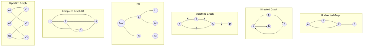
Undirected graph: Edges have no direction. An edge {u, v} connects u and v symmetrically.
Directed graph (digraph): Edges have direction. An edge (u, v) goes from u to v (u → v). Here (u, v) ≠ (v, u).
Weighted graph: Each edge has an associated numerical value (weight, cost, distance, capacity).
Simple graph: No self-loops (edges from a vertex to itself) and no multiple edges between the same pair of vertices.
Multigraph: Allows multiple edges between the same pair of vertices.
Pseudograph: Allows both multiple edges and self-loops.
Complete graph Kₙ: Every pair of vertices is connected. Has C(n, 2) = n(n-1)/2 edges.
Bipartite graph: Vertices can be divided into two disjoint sets U and V such that every edge connects a vertex in U to one in V. Equivalently: the graph is 2-colorable (no odd cycles).
Complete bipartite graph Kₘ,ₙ: Every vertex in U is connected to every vertex in V. Has m × n edges.
Degree
Undirected Graphs
The degree of vertex v, written deg(v), is the number of edges incident to v. A self-loop contributes 2 to the degree.
Handshaking Lemma: The sum of all vertex degrees equals twice the number of edges.
Σᵥ∈V deg(v) = 2|E|
Corollary: The number of vertices with odd degree is always even.
Proof: Σ deg(v) = 2|E| is even. If there were an odd number of odd-degree vertices, the sum would be odd. Contradiction. ∎
Directed Graphs
- In-degree deg⁻(v): Number of edges coming into v.
- Out-degree deg⁺(v): Number of edges going out of v.
Σᵥ deg⁻(v) = Σᵥ deg⁺(v) = |E|
Degree Sequence
The degree sequence is the list of degrees sorted in non-increasing order.
Example: A graph with degrees [3, 3, 2, 2, 2] has 5 vertices and (3+3+2+2+2)/2 = 6 edges.
Erdos-Gallai Theorem: A non-increasing sequence d₁ ≥ d₂ ≥ ... ≥ dₙ is a valid degree sequence of a simple graph iff:
- Σ dᵢ is even.
- For each k = 1, ..., n: Σᵢ₌₁ᵏ dᵢ ≤ k(k-1) + Σᵢ₌ₖ₊₁ⁿ min(dᵢ, k).
Graph Representations
Adjacency Matrix
An n × n matrix A where Aᵢⱼ = 1 if edge (i, j) exists, 0 otherwise.
For undirected graphs: A is symmetric (Aᵢⱼ = Aⱼᵢ).
Space: O(n²). Edge lookup: O(1). List neighbors: O(n). Good for: Dense graphs, matrix-based algorithms (spectral methods, Floyd-Warshall).
Example:
Graph: 1-2, 2-3, 1-3

    1  2  3
1 [ 0  1  1 ]
2 [ 1  0  1 ]
3 [ 1  1  0 ]
Property: Aᵏ[i][j] = number of walks of length k from i to j.
Adjacency List
For each vertex, store a list of its neighbors.
Space: O(n + m) where m = |E|. Edge lookup: O(deg(v)). List neighbors: O(deg(v)). Good for: Sparse graphs, BFS/DFS, most algorithms.
1: [2, 3]
2: [1, 3]
3: [1, 2]
Edge List
Simply a list of all edges: [(u₁, v₁), (u₂, v₂), ...].
Space: O(m). Good for: Kruskal's algorithm, simple storage, input/output.
Incidence Matrix
An n × m matrix B where Bᵢⱼ = 1 if vertex i is incident to edge j.
For directed graphs: Bᵢⱼ = -1 if edge j leaves vertex i, +1 if it enters.
Space: O(n × m). Rarely used in practice.
Graph Isomorphism
Two graphs G₁ = (V₁, E₁) and G₂ = (V₂, E₂) are isomorphic (G₁ ≅ G₂) if there exists a bijection f: V₁ → V₂ such that (u, v) ∈ E₁ iff (f(u), f(v)) ∈ E₂.
In other words: They have the same structure, just with different vertex labels.
Necessary Conditions (Quick Rejection)
If G₁ ≅ G₂, then:
- Same number of vertices
- Same number of edges
- Same degree sequence
- Same number of connected components
- Same cycle structure
These are necessary but not sufficient — non-isomorphic graphs can share all these properties.
Example: The Petersen graph and a graph with the same degree sequence (3-regular, 10 vertices, 15 edges) might not be isomorphic.
Computational Complexity
Graph isomorphism is in NP but not known to be in P or NP-complete. Babai (2015) showed it can be solved in quasi-polynomial time: n^O(log n).
Subgraphs
A subgraph H of G: V(H) ⊆ V(G) and E(H) ⊆ E(G), where endpoints of edges in H are in V(H).
An induced subgraph G[S] for S ⊆ V: Contains all vertices in S and all edges of G between vertices in S.
A spanning subgraph: V(H) = V(G) (uses all vertices, possibly fewer edges).
Complements
The complement G̅ of a simple graph G = (V, E) has the same vertex set V and edges:
E(G̅) = {(u, v) | u, v ∈ V, u ≠ v, (u, v) ∉ E(G)}
Properties:
- G̅̅ = G
- |E(G)| + |E(G̅)| = C(n, 2) = n(n-1)/2
- G is connected or G̅ is connected (or both)
A graph is self-complementary if G ≅ G̅. Examples: P₄ (path on 4 vertices), C₅ (cycle on 5 vertices).
Special Graph Families
Paths and Cycles
- Path Pₙ: n vertices in a line. n-1 edges.
- Cycle Cₙ: n vertices in a loop. n edges. Requires n ≥ 3.
Regular Graphs
A graph is k-regular if every vertex has degree k.
- 0-regular: isolated vertices
- 1-regular: perfect matching
- 2-regular: disjoint union of cycles
- 3-regular: cubic graph (e.g., Petersen graph, K₃,₃)
- (n-1)-regular on n vertices: complete graph Kₙ
Trees
A tree is a connected acyclic graph. Key properties:
- n vertices, n-1 edges
- Exactly one path between any two vertices
- Removing any edge disconnects it
- Adding any edge creates exactly one cycle
Hypercube Graphs
Qₙ: 2ⁿ vertices (one per n-bit string), edges between strings differing in exactly one bit.
- Q₁ = K₂
- Q₂ = C₄ (square)
- Q₃ = cube
- Qₙ is n-regular, bipartite, has 2ⁿ vertices and n·2ⁿ⁻¹ edges
Petersen Graph
A famous 3-regular graph with 10 vertices and 15 edges. It is a counterexample for many graph theory conjectures and has no Hamiltonian cycle, is non-planar (but is a minor-minimal non-planar graph for the Petersen family), and has chromatic number 3.
Operations on Graphs
Union: G₁ ∪ G₂ = (V₁ ∪ V₂, E₁ ∪ E₂).
Intersection: G₁ ∩ G₂ = (V₁ ∩ V₂, E₁ ∩ E₂).
Cartesian product: G₁ □ G₂. Vertices: V₁ × V₂. Edge between (u₁, u₂) and (v₁, v₂) if u₁ = v₁ and (u₂, v₂) ∈ E₂, or u₂ = v₂ and (u₁, v₁) ∈ E₁.
Example: Pₘ □ Pₙ = grid graph. Cₘ □ Cₙ = torus.
Graph minor: H is a minor of G if H can be obtained from G by deleting vertices, deleting edges, and contracting edges.
Edge contraction: Merge the endpoints of an edge into a single vertex.
Real-World Applications
- Social networks: Users are vertices, friendships are edges. Degree = number of friends. Community detection = graph clustering.
- Computer networks: Routers are vertices, links are edges. Shortest path algorithms find routing. Network topology design uses graph properties.
- Web: Pages are vertices, hyperlinks are directed edges. PageRank operates on this digraph. Web crawling is graph traversal.
- Dependencies: Build systems (make, bazel), package managers (npm, cargo), task scheduling — all use directed acyclic graphs (DAGs).
- Maps and navigation: Intersections are vertices, roads are weighted edges. GPS routing = shortest path.
- Databases: Entity-relationship diagrams, query plan graphs, join graphs.
- Compilers: Control flow graphs, data flow graphs, interference graphs (register allocation), call graphs.
- Biology: Protein interaction networks, metabolic networks, phylogenetic trees.
- Circuit design: Logic gates are vertices, wires are edges.