Channel Coding

Channel Capacity

The channel capacity of a discrete memoryless channel (DMC) is the maximum rate at which information can be transmitted with arbitrarily low error probability:

$C = \max_{p(x)} I(X; Y)$

where the maximization is over input distributions. This is a convex optimization problem (mutual information is concave in $p(x)$ for fixed channel). The Blahut-Arimoto algorithm computes $C$ iteratively via alternating maximization.

For a channel with input $X$, output $Y$, and transition probabilities $p(y|x)$:

• $C \geq 0$, with $C = 0$ iff $X$ and $Y$ are independent for all input distributions
• $C \leq \min(\log|\mathcal{X}|, \log|\mathcal{Y}|)$
• Feedback does not increase capacity for DMCs (but simplifies coding)

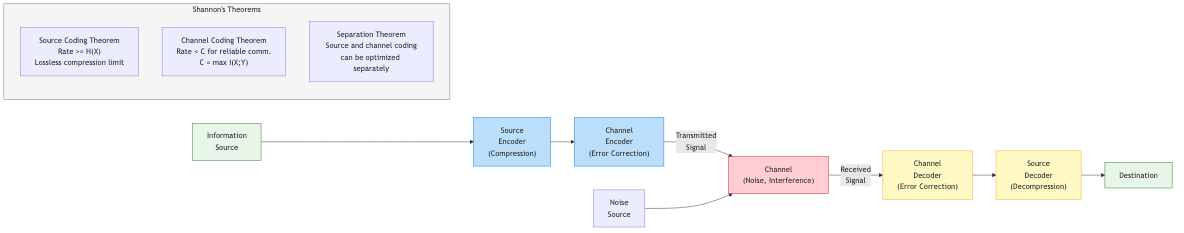
Shannon's Channel Coding Theorem (Second Theorem)

Achievability: For any rate $R < C$, there exists a sequence of $(2^{nR}, n)$ codes with probability of error $P_e^{(n)} \to 0$ as $n \to \infty$.

Converse: For any rate $R > C$, any sequence of codes has $P_e^{(n)} \to 1$.

Error exponent (reliability function): for $R < C$, the best achievable error probability decays as $P_e^{(n)} \sim 2^{-nE(R)}$ where $E(R) > 0$. The random coding exponent provides a lower bound; the sphere-packing exponent provides an upper bound. They coincide at high rates (above the critical rate).

Shannon's proof used random coding: generate $2^{nR}$ codewords i.i.d. from the capacity-achieving input distribution, decode via joint typicality. Non-constructive but establishes the fundamental limit.

Binary Symmetric Channel (BSC)

Flips each bit independently with probability $p$ (crossover probability).

$C_{\text{BSC}} = 1 - H_b(p)$

Achieved by uniform input distribution. At $p = 0$: $C = 1$ bit. At $p = 1/2$: $C = 0$ (completely noisy).

Binary Erasure Channel (BEC)

Each bit is either received correctly or erased (marked as unknown) with probability $\epsilon$.

$C_{\text{BEC}} = 1 - \epsilon$

The BEC is analytically tractable and serves as the primary channel model for analyzing LDPC and polar codes. Capacity is achieved by uniform input. ML decoding reduces to solving linear equations over GF(2).

Additive White Gaussian Noise (AWGN) Channel

Continuous-valued: $Y = X + Z$ where $Z \sim \mathcal{N}(0, N)$, with average power constraint $\frac{1}{n}\sum x_i^2 \leq P$.

$C_{\text{AWGN}} = \frac{1}{2}\log\left(1 + \frac{P}{N}\right) \quad \text{bits/channel use}$

This is the Shannon-Hartley theorem. With bandwidth $W$ and noise spectral density $N_0/2$:

$C = W \log_2\left(1 + \frac{P}{N_0 W}\right) \quad \text{bits/second}$

In the wideband limit ($W \to \infty$): $C \to \frac{P}{N_0 \ln 2}$ (power-limited regime). The capacity-achieving input distribution is Gaussian.

Shannon limit: the minimum $E_b/N_0$ for reliable communication is $-1.59$ dB, achieved as $R \to 0$.

Linear Block Codes

An $(n, k)$ linear code over GF($q$) is a $k$-dimensional subspace of GF($q$)^n. Rate $R = k/n$.

• Generator matrix $G$: $k \times n$, codeword $c = uG$ for message $u$
• Parity-check matrix $H$: $(n-k) \times n$, $Hc^T = 0$ for all codewords
• Minimum distance $d_{\min}$: minimum Hamming weight of nonzero codewords
• Can detect $d_{\min} - 1$ errors and correct $\lfloor(d_{\min}-1)/2\rfloor$ errors
• Singleton bound: $d_{\min} \leq n - k + 1$. Codes achieving equality are MDS (maximum distance separable)

Syndrome decoding: compute $s = Hy^T$; syndrome determines the error pattern (for errors within correction capability).

Hamming Codes

Parameters: $(2^r - 1, 2^r - 1 - r, 3)$ for any $r \geq 2$. Rate $R = 1 - r/(2^r - 1) \to 1$.

• Corrects any single-bit error
• Perfect code: every vector is within Hamming distance 1 of exactly one codeword (meets Hamming/sphere-packing bound)
• Parity-check matrix columns are all nonzero $r$-bit vectors
• Extended Hamming: append overall parity bit, yielding $(2^r, 2^r - 1 - r, 4)$, used in ECC memory (SECDED)

Reed-Solomon Codes

$(n, k, n-k+1)$ MDS codes over GF($q$) with $n \leq q$, typically $q = 2^m$, $n = q - 1 = 2^m - 1$.

• Corrects up to $t = \lfloor(n-k)/2\rfloor$ symbol errors
• Particularly effective against burst errors (each symbol is $m$ bits)
• Encoding: evaluate message polynomial at $n$ points, or systematic via polynomial division
• Decoding: Berlekamp-Massey algorithm (finds error-locator polynomial), then Chien search (finds error locations), then Forney's formula (finds error values). Complexity $O(nt)$

Applications: CDs, DVDs, QR codes, deep-space communication, RAID-6, digital television. Often concatenated with an inner code (e.g., convolutional) for compound error correction.

Convolutional Codes

Encode a continuous stream of bits using shift registers. Characterized by:

• Rate $R = k/n$ (input/output bits per time step)
• Constraint length $K$: number of shift register stages + 1
• Memory $m = K - 1$
• Generator polynomials: define connections from shift register to output

The code has $2^m$ states, naturally represented as a trellis. State transitions define a finite-state machine.

Viterbi Algorithm

Maximum-likelihood sequence decoding via dynamic programming on the trellis.

• Complexity: $O(2^m \cdot n)$ per decoded bit (exponential in constraint length)
• Optimal (ML) for the given code
• Practical constraint lengths: $K \leq 10$ (state space $2^m \leq 512$)
• Traceback: store surviving paths, output decision after traceback depth $\approx 5K$
• Soft-decision Viterbi: uses channel LLRs instead of hard bits, gaining ~2 dB

BCJR Algorithm

Computes a posteriori probabilities (APP) for each bit via forward-backward on the trellis. Essential for iterative (turbo) decoding. Complexity similar to Viterbi but computes marginals rather than MAP sequence.

Turbo Codes

Berrou, Glavieux, Thitimajshima (1993). Two parallel concatenated convolutional codes with a random interleaver between them.

Encoder: systematic bits + parity from encoder 1 + parity from encoder 2 (fed interleaved data). Rate $\approx 1/3$ before puncturing.

Iterative decoding: two BCJR decoders exchange extrinsic information (soft bit estimates) iteratively. Each decoder uses the other's output as prior information. Typically 6-18 iterations.

Performance:

• Approach capacity within 0.5 dB on AWGN at moderate block lengths (~$10^4$)
• First practical near-capacity codes
• Used in 3G/4G cellular (UMTS, LTE), deep-space (CCSDS)
• Error floor: residual errors at high SNR due to low-weight codewords from specific interleaver patterns

LDPC Codes

Low-density parity-check codes (Gallager, 1962; rediscovered by MacKay & Neal, 1996).

Defined by a sparse parity-check matrix $H$ with few 1s per row/column. Represented by a Tanner graph (bipartite: variable nodes and check nodes).

Regular LDPC$(d_v, d_c)$: each variable node has degree $d_v$, each check node has degree $d_c$. Rate $R \geq 1 - d_v/d_c$.

Irregular LDPC: variable and check node degrees follow optimized distributions $(\lambda(x), \rho(x))$. Density evolution (Richardson-Urbanke) tracks message distributions through iterations to find the decoding threshold. Optimized irregular codes achieve within 0.0045 dB of capacity on BEC.

Belief Propagation Decoding

Message-passing on the Tanner graph:

1. Variable-to-check messages: sum of incoming check-to-variable messages (in LLR domain)
2. Check-to-variable messages: $\tanh^{-1}\left(\prod \tanh(m/2)\right)$ or min-sum approximation
3. Iterate until convergence or max iterations (typically 50-100)

Exact on trees (cycle-free graphs); approximate on graphs with cycles. Min-sum and offset min-sum are practical low-complexity approximations.

Decoding complexity: $O(n \cdot \bar{d} \cdot I)$ where $\bar{d}$ is average degree and $I$ is iteration count. Highly parallelizable.

Used in: DVB-S2, 802.11n/ac/ax (WiFi), 5G NR (data channels), 10GBASE-T Ethernet.

Polar Codes

Arikan (2009). First provably capacity-achieving codes with explicit construction and $O(n \log n)$ encoding/decoding complexity.

Channel polarization: apply recursive butterfly transform $G_N = B_N F^{\otimes n}$ where $F = \begin{bmatrix} 1 & 0 \\ 1 & 1 \end{bmatrix}$. As $N = 2^n \to \infty$, synthetic channels polarize: fraction $C$ become perfect (capacity 1), fraction $1-C$ become useless (capacity 0).

Encoding: place information bits on the $K$ most reliable synthetic channels, fix remaining $N-K$ positions to known values ("frozen bits").

Successive cancellation (SC) decoding: decode bits sequentially in order $u_1, u_2, \ldots, u_N$, using previously decoded bits. Complexity $O(N \log N)$.

SC List (SCL) decoding: maintain $L$ candidate paths, prune after each bit decision. With CRC-aided selection (CA-SCL), performance matches or exceeds turbo/LDPC at short-to-moderate block lengths. Used in 5G NR control channels.

Polarization-adjusted convolutional (PAC) codes: concatenate convolutional pre-transform with polar transform, achieving near-optimal performance at short block lengths.

Capacity-Achieving Code Families

| Code Family | Capacity-Achieving? | Complexity (Encoding) | Complexity (Decoding) | Practical Gap to Capacity | |---|---|---|---|---| | Random codes | Yes (Shannon) | Exponential | Exponential | Theoretical only | | LDPC (irregular) | Yes (BEC, near for AWGN) | $O(n)$ | $O(n \cdot I)$ | < 0.1 dB | | Polar | Yes (any symmetric DMC) | $O(n \log n)$ | $O(n \log n)$ (SC) | ~0.5 dB (SC), <0.1 dB (SCL) | | Turbo | Empirically near | $O(n)$ | $O(n \cdot I)$ | ~0.3-0.5 dB | | Spatially coupled LDPC | Yes (threshold saturation) | $O(n)$ | $O(n \cdot I)$ | < 0.05 dB |

Threshold saturation (spatially coupled LDPC): coupling regular LDPC codes in a chain causes the BP threshold to equal the MAP threshold, which equals capacity for BMS channels.

Coded Modulation

For bandwidth-limited channels, combine coding with higher-order modulation:

• Trellis-coded modulation (TCM): Ungerboeck (1982). Combine convolutional code with set-partitioning of signal constellation. Achieves coding gain without bandwidth expansion
• Bit-interleaved coded modulation (BICM): separate binary code from modulation via bit-level interleaving. Simpler, flexible, near-optimal with iterative demapping (BICM-ID)
• Multilevel coding (MLC): protect different bit levels of modulation with different-rate codes. Optimal with multistage decoding

Rateless Codes

Transmit potentially infinite stream of coded symbols; receiver collects enough for decoding.

• LT codes (Luby, 2002): first practical rateless codes. Random sparse bipartite graph, peeling decoder. Require $(1+\epsilon)k$ symbols for $k$ information symbols. Robust Soliton distribution optimizes degree profile
• Raptor codes (Shokrollahi, 2006): concatenate high-rate LDPC pre-code with LT code. Linear-time encoding/decoding, approach capacity of BEC. Standardized in 3GPP MBMS, ATSC 3.0
• Fountain codes: general term for rateless codes. Particularly useful for broadcast/multicast (no feedback needed)

Sphere Packing and Fundamental Limits

The sphere-packing (Hamming) bound: $M \cdot V(n, t) \leq 2^n$ where $V(n,t) = \sum_{i=0}^t \binom{n}{i}$ is the volume of a Hamming sphere of radius $t$. Perfect codes meet this bound: Hamming codes, Golay codes, trivial codes.

The Gilbert-Varshamov bound shows good codes exist: there exists an $(n, k, d)$ code if $\sum_{i=0}^{d-2}\binom{n-1}{i} < 2^{n-k}$.

Plotkin bound, Elias-Bassalygo bound, and the linear programming bound (Delsarte) provide tighter limits in different parameter regimes.