Matrix Decompositions

Matrix decompositions (factorizations) express a matrix as a product of simpler matrices. They are the computational backbone of numerical linear algebra — solving systems, computing eigenvalues, least squares, and compression.

Matrix Decomposition Hierarchy

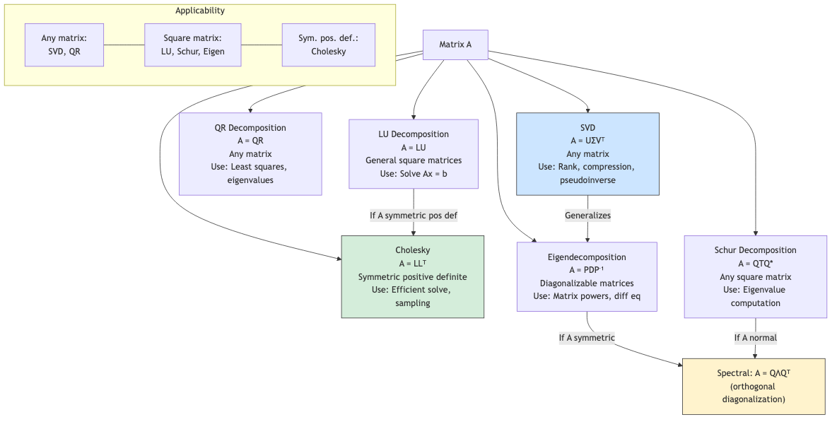
LU Decomposition

Factor A into a lower triangular L and upper triangular U:

A = LU

L has 1s on the diagonal (unit lower triangular). U is the row echelon form.

With Partial Pivoting

In practice, row swaps are needed for numerical stability:

PA = LU

where P is a permutation matrix.

Algorithm

Gaussian elimination records multipliers in L:

For k = 1 to n-1:
    For i = k+1 to n:
        L[i][k] = A[i][k] / A[k][k]
        For j = k to n:
            A[i][j] -= L[i][k] * A[k][j]
U = resulting upper triangular

Time: O(2n³/3).

Solving Ax = b with LU

Factor A = LU (once): O(n³).
Solve Ly = b by forward substitution: O(n²).
Solve Ux = y by back substitution: O(n²).

For multiple right-hand sides, LU is much more efficient than re-doing Gaussian elimination.

LDU Decomposition

Separate the diagonal: A = LDU where L is unit lower triangular, D is diagonal, U is unit upper triangular.

Cholesky Decomposition

For symmetric positive definite (SPD) matrices:

A = LLᵀ

where L is lower triangular with positive diagonal entries. Unique.

Algorithm:

For j = 1 to n:
    L[j][j] = √(A[j][j] - Σₖ₌₁ʲ⁻¹ L[j][k]²)
    For i = j+1 to n:
        L[i][j] = (A[i][j] - Σₖ₌₁ʲ⁻¹ L[i][k]·L[j][k]) / L[j][j]

Time: O(n³/3) — half the cost of LU.

Applications: Solving SPD systems (covariance matrices, kernel matrices), sampling from multivariate Gaussians, computing determinants (det(A) = (Π L[i][i])²).

Existence: A = LLᵀ exists iff A is symmetric positive definite. If A[j][j] - Σ L[j][k]² ≤ 0 during computation, A is not SPD.

QR Decomposition

Factor A into an orthogonal Q and upper triangular R:

A = QR

Covered in the inner product spaces file. Three methods:

Gram-Schmidt: Conceptually simple, numerically unstable.
Householder reflections: Numerically stable, most common.
Givens rotations: For sparse matrices.

Singular Value Decomposition (SVD)

SVD Geometric Interpretation

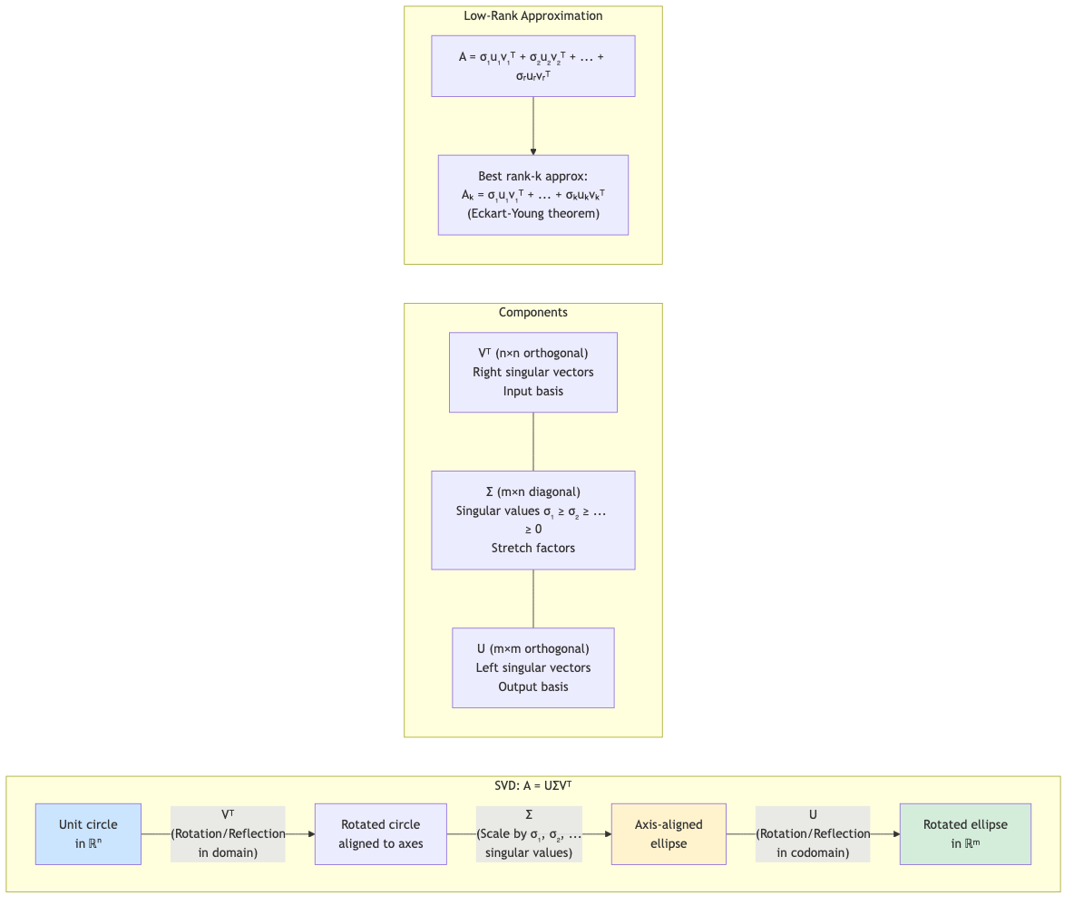
The most important matrix decomposition. Every m × n matrix A (real or complex) can be factored as:

A = UΣVᵀ

where:

U ∈ ℝᵐˣᵐ is orthogonal (left singular vectors)
Σ ∈ ℝᵐˣⁿ is diagonal with non-negative entries σ₁ ≥ σ₂ ≥ ... ≥ σᵣ > 0 (singular values)
V ∈ ℝⁿˣⁿ is orthogonal (right singular vectors)
r = rank(A)

Relationship to Eigenvalues

σᵢ² are the eigenvalues of AᵀA (and AAᵀ).
Columns of V are eigenvectors of AᵀA.
Columns of U are eigenvectors of AAᵀ.
σᵢ = √λᵢ (singular values are square roots of eigenvalues of AᵀA).

Compact SVD

Only keep the r non-zero singular values:

A = U_r Σ_r V_r^T

where U_r is m × r, Σ_r is r × r, V_r is n × r.

Truncated SVD (Low-Rank Approximation)

Keep only the k largest singular values (k < r):

A_k = U_k Σ_k V_k^T

Eckart-Young-Mirsky Theorem: A_k is the best rank-k approximation to A in both Frobenius and spectral norms:

‖A - A_k‖_F = √(σ_{k+1}² + ... + σ_r²)
‖A - A_k‖₂ = σ_{k+1}

No other rank-k matrix is closer. This is the theoretical foundation of PCA, dimensionality reduction, and data compression.

SVD Properties

rank(A) = number of non-zero singular values
‖A‖₂ = σ₁ (largest singular value = spectral norm)
‖A‖_F = √(Σ σᵢ²) (Frobenius norm)
Condition number: κ(A) = σ₁/σᵣ (measures numerical sensitivity)
Pseudoinverse: A⁺ = VΣ⁺Uᵀ where Σ⁺ inverts the non-zero singular values

Computing SVD

Reduce to bidiagonal form via Householder reflections: O(mn²).
Apply iterative methods (Golub-Kahan, divide-and-conquer) to the bidiagonal matrix.
Total: O(mn²) for an m × n matrix (m ≥ n).

For large sparse matrices, compute only the top k singular values: randomized SVD, Lanczos/Arnoldi.

Polar Decomposition

Every matrix A can be written as:

A = UP

where U is orthogonal (or unitary) and P is symmetric positive semidefinite.

P = √(AᵀA) (the "stretch" part)
U = AP⁻¹ (the "rotation" part, if A is invertible)

This separates rotation from stretching, analogous to polar form of complex numbers.

Schur Decomposition

Every square matrix A can be factored as:

A = QTQ*

where Q is unitary and T is upper triangular. The diagonal of T contains the eigenvalues.

For real matrices with only real eigenvalues, Q can be real orthogonal and T real upper triangular.

For real matrices with complex eigenvalues, the real Schur form uses 2×2 blocks on the diagonal for complex conjugate eigenvalue pairs.

The QR algorithm converges to the Schur form.

Jordan Normal Form

Every matrix A over ℂ is similar to a Jordan normal form J:

A = PJP⁻¹

where J is block-diagonal with Jordan blocks:

Jₖ(λ) = [λ  1  0  ...  0]
         [0  λ  1  ...  0]
         [0  0  λ  ...  0]
         [⋮  ⋮  ⋮   ⋱   1]
         [0  0  0  ...  λ]

Each Jordan block has eigenvalue λ on the diagonal and 1s on the superdiagonal.

When Jordan Form = Diagonal

If all Jordan blocks are 1×1, J is diagonal. This happens iff A is diagonalizable (geometric multiplicity = algebraic multiplicity for all eigenvalues).

Practical Notes

Jordan form is numerically unstable — small perturbations can change the Jordan structure. In practice, Schur form is preferred for computation.

Jordan form is primarily a theoretical tool: understanding matrix powers, exponentials, and canonical structure.

Matrix Exponential

e^{tJ_k(λ)} = e^{tλ} [1     t    t²/2  ...  t^(k-1)/(k-1)!]
                       [0     1    t     ...  t^(k-2)/(k-2)!]
                       [⋮     ⋮    ⋮      ⋱           ⋮     ]
                       [0     0    0     ...        1        ]

So e^{tA} = P e^{tJ} P⁻¹. Used in solving systems of differential equations x' = Ax.

Summary of Decompositions

| Decomposition | Form | Requirements | Cost | Primary Use | |---|---|---|---|---| | LU | A = LU | Square (with pivoting: any) | O(n³) | Solve Ax = b | | Cholesky | A = LLᵀ | SPD | O(n³/3) | SPD systems, sampling | | QR | A = QR | Any (m ≥ n) | O(mn²) | Least squares, eigenvalues | | Eigendecomposition | A = PDP⁻¹ | Square, diagonalizable | O(n³) | Spectral analysis | | SVD | A = UΣVᵀ | Any | O(mn²) | Low-rank approx, pseudoinverse | | Schur | A = QTQ* | Square | O(n³) | Eigenvalues (stable) | | Jordan | A = PJP⁻¹ | Square (over ℂ) | Unstable | Theoretical | | Polar | A = UP | Any | O(n³) | Rotation extraction |

Real-World Applications

LU: Solving large linear systems in circuit simulation, structural analysis, fluid dynamics.
Cholesky: Gaussian process regression, portfolio optimization, Kalman filters.
QR: Least squares regression, QR algorithm for eigenvalues, signal processing.
SVD: Image compression (keep top-k singular values), recommendation systems (matrix completion), latent semantic analysis, noise reduction, pseudoinverse for ill-conditioned systems.
PCA: SVD of centered data gives principal components.
Matrix exponential: Solving ODEs, Markov chain analysis, quantum mechanics (time evolution).