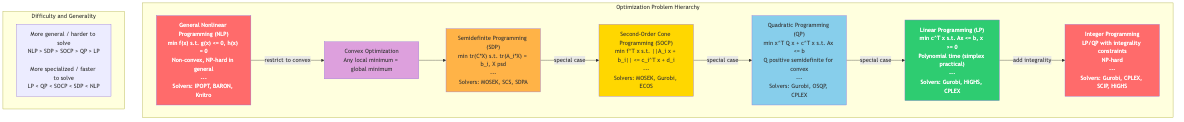
Convex Optimization

Optimization problem hierarchy

Convex Sets and Functions

A set C is convex if for all x, y in C and theta in [0, 1]: theta*x + (1-theta)*y in C. Key examples: hyperplanes, halfspaces, polyhedra, ellipsoids, norm balls, positive semidefinite cone.

A function f: R^n -> R is convex if dom(f) is convex and for all x, y in dom(f):

f(theta*x + (1-theta)*y) <= theta*f(x) + (1-theta)*f(y)

Equivalent characterizations:

First-order: f(y) >= f(x) + grad(f(x))^T (y - x) for all x, y (the function lies above its tangent hyperplanes).
Second-order: the Hessian H(x) is positive semidefinite everywhere.

Strongly convex (parameter mu > 0): f(y) >= f(x) + grad(f(x))^T (y-x) + (mu/2) ||y-x||^2. This guarantees a unique minimizer and faster convergence.

L-smooth: ||grad(f(x)) - grad(f(y))|| <= L ||x-y|| for all x, y. Equivalently, f(y) <= f(x) + grad(f(x))^T (y-x) + (L/2) ||y-x||^2.

The condition number kappa = L/mu governs convergence rates.

Standard Convex Optimization Problem

minimize    f(x)
subject to  g_i(x) <= 0,   i = 1,...,m   (convex)
            h_j(x) = 0,    j = 1,...,p   (affine)

Any local minimum is a global minimum. This is the fundamental property that makes convex optimization tractable.

Gradient Descent

The workhorse of unconstrained convex optimization.

x_{k+1} = x_k - alpha_k * grad(f(x_k))

| Setting | Step size | Rate | Iterations to epsilon | |---------|-----------|------|----------------------| | Convex, L-smooth | 1/L | O(1/k) | O(L/epsilon) | | mu-strongly convex, L-smooth | 2/(L+mu) | O((1 - mu/L)^k) | O(kappa * ln(1/epsilon)) |

Constant step size alpha = 1/L is safe when L is known.
Line search (Armijo/backtracking): find alpha satisfying f(x - alpha*grad) <= f(x) - c*alpha*||grad||^2. Adaptive and practical.
Exact line search: alpha = argmin f(x - alpha*grad). Rarely used except for quadratics.

Nesterov's Accelerated Gradient

Achieves the optimal rate for first-order methods on smooth convex problems.

y_{k+1} = x_k - (1/L) * grad(f(x_k))
x_{k+1} = y_{k+1} + (k-1)/(k+2) * (y_{k+1} - y_k)

Convergence Rates

| Setting | Rate | Lower bound match? | |---------|------|--------------------| | Convex, L-smooth | O(1/k^2) | Yes (Nesterov 1983) | | Strongly convex, L-smooth | O((1 - sqrt(mu/L))^k) | Yes |

The momentum term (k-1)/(k+2) provides acceleration. For strongly convex problems, use a constant momentum (sqrt(kappa) - 1)/(sqrt(kappa) + 1).

Proximal Gradient Methods

For composite problems: minimize f(x) + g(x) where f is smooth and g is convex but possibly nonsmooth (e.g., L1 norm).

The proximal operator of g:

prox_{alpha*g}(v) = argmin_x { g(x) + (1/(2*alpha)) ||x - v||^2 }

Proximal gradient step:

x_{k+1} = prox_{alpha/L, g}( x_k - (1/L) * grad(f(x_k)) )

Key proximal operators:

g(x) = lambda * ||x||_1: soft thresholding (ISTA for LASSO)
g(x) = indicator of convex set C: projection onto C
g(x) = lambda * ||X||_*: singular value soft thresholding

FISTA: accelerated proximal gradient, achieves O(1/k^2) rate.

Projected Gradient Descent

Special case of proximal gradient where g is the indicator function of a convex set C.

x_{k+1} = proj_C( x_k - alpha_k * grad(f(x_k)) )

Convergence matches standard gradient descent rates. The bottleneck is the projection step, which must be efficient. Closed-form projections exist for boxes, simplices, L2 balls, halfspaces, and affine subspaces.

Mirror Descent

Generalizes projected gradient by replacing the Euclidean distance with a Bregman divergence D_phi:

x_{k+1} = argmin_x { <grad(f(x_k)), x> + (1/alpha_k) * D_phi(x, x_k) }

When phi(x) = (1/2)||x||^2, this recovers projected gradient. For the simplex with phi(x) = sum x_i ln(x_i) (negative entropy), mirror descent gives the exponentiated gradient update, which is dimension-free in its convergence bound.

Useful when the geometry of the constraint set is better captured by a non-Euclidean distance.

Frank-Wolfe (Conditional Gradient)

For minimizing a smooth function over a compact convex set C:

s_k = argmin_{s in C} <grad(f(x_k)), s>       (linear minimization oracle)
x_{k+1} = x_k + gamma_k * (s_k - x_k)         (gamma_k = 2/(k+2))

Advantages: projection-free (only requires a linear oracle over C), iterates remain in C, and solutions are sparse (convex combinations of vertices). Rate: O(1/k) for smooth convex f, which is tight for this oracle model.

Applications: matrix completion (nuclear norm ball), structured sparsity, traffic assignment.

ADMM (Alternating Direction Method of Multipliers)

Solves problems of the form: minimize f(x) + g(z) subject to Ax + Bz = c.

Augmented Lagrangian with penalty rho:

x_{k+1} = argmin_x { f(x) + (rho/2) ||Ax + Bz_k - c + u_k||^2 }
z_{k+1} = argmin_z { g(z) + (rho/2) ||Ax_{k+1} + Bz - c + u_k||^2 }
u_{k+1} = u_k + Ax_{k+1} + Bz_{k+1} - c

ADMM decomposes the problem into subproblems that are often easier to solve. Convergence rate is O(1/k) in general. Widely used in distributed optimization, signal processing, and machine learning (LASSO, consensus problems).

Practical Considerations

Penalty parameter rho: critical for convergence speed. Adaptive schemes (residual balancing) help.
Over-relaxation: replace Ax_{k+1} with alphaAx_{k+1} - (1-alpha)(Bz_k - c) with alpha in (1, 1.8) for speedup.
Stopping criteria: primal residual ||Ax + Bz - c|| and dual residual ||rho * B^T (z_{k+1} - z_k)|| both below tolerance.

Summary of Rates

| Method | Smooth convex | Strongly convex | |--------|--------------|-----------------| | Gradient descent | O(1/k) | O(exp(-k/kappa)) | | Accelerated gradient | O(1/k^2) | O(exp(-k/sqrt(kappa))) | | Proximal gradient | O(1/k) | O(exp(-k/kappa)) | | Frank-Wolfe | O(1/k) | O(1/k) | | Mirror descent | O(1/sqrt(k)) | O(exp(-k*mu)) |

Connections

Duality theory underlying these methods (→ 04-duality-and-kkt.md).
Conic optimization as structured convex optimization (→ 05-conic-programming.md).
Newton and quasi-Newton for faster local convergence (→ 06-nonlinear-programming.md).
Stochastic variants of gradient methods (→ 08-stochastic-optimization.md).