Optimization Solvers and Modeling
Solver Landscape
Commercial Solvers
Gurobi
- LP, MIP, QP, QCQP, SOCP (via barrier), bilinear.
- State-of-the-art MIP performance (consistently top in benchmarks).
- Parallel branch and cut, advanced presolve, heuristics, cutting planes.
- APIs: Python (gurobipy), C, C++, Java, .NET, R, MATLAB.
- Free academic licenses available.
CPLEX (IBM)
- LP, MIP, QP, QCQP, SOCP, constraint programming (CP Optimizer).
- Comparable to Gurobi on MIP. CP Optimizer excels at scheduling.
- Tight integration with IBM Decision Optimization platform.
- APIs: Python (docplex), C, C++, Java, .NET.
MOSEK
- LP, SOCP, SDP, exponential cone, power cone, MIP.
- Best-in-class for conic optimization, especially SDP and SOCP.
- Interior point method with advanced numerical linear algebra.
- APIs: Python (Fusion), C, Java, .NET, MATLAB.
- Free academic licenses.
XPRESS (FICO)
- LP, MIP, QP, QCQP, SOCP, nonlinear.
- Strong MIP solver, competitive with Gurobi/CPLEX.
- Used extensively in financial services and logistics.
Open-Source Solvers
HiGHS
- LP, MIP, QP.
- Best open-source LP/MIP solver (as of 2025). Simplex and IPM for LP.
- Written in C++ with Python bindings. Actively developed.
- Performance approaching commercial solvers on many LP/MIP instances.
SCIP
- MIP, MINLP, constraint integer programming.
- Most versatile academic solver. Highly extensible plugin architecture.
- Supports nonlinear constraints, indicator constraints, SOS.
- Often used as a research platform for new MIP techniques.
GLPK
- LP, MIP.
- Mature, simple, widely available. Performance below HiGHS/SCIP.
- Good for educational use and small problems.
CBC (COIN-OR)
- LP (via CLP), MIP.
- Solid open-source MIP solver. Being overtaken by HiGHS.
SCS (Splitting Conic Solver)
- LP, SOCP, SDP, exponential/power cones.
- First-order method (ADMM-based). Scales to large problems but with moderate accuracy.
- Default backend for CVXPY.
OSQP
- Convex QP.
- ADMM-based, very fast for moderate-accuracy solutions. Ideal for embedded/real-time optimization (MPC).
IPOPT
- General nonlinear programming (NLP).
- Interior point method. Requires first and second derivatives (or approximations).
- De facto standard open-source NLP solver.
BARON
- Global optimization for nonconvex MINLP.
- Spatial branch and bound with convex relaxations.
Specialized Solvers
| Domain | Solver | Method |
|---|---|---|
| SAT/MaxSAT | CaDiCaL, Kissat, RC2 | CDCL, core-guided |
| CP | OR-Tools CP-SAT, Chuffed | Lazy clause generation |
| Convex (first-order) | ProximalOperators.jl, ECOS | Proximal, IPM |
| Bayesian optimization | BoTorch, Ax | GP + acquisition |
| Derivative-free | COBYLA, NOMAD, Py-BOBYQA | Model-based, direct search |
Modeling Languages and Frameworks
CVXPY (Python)
Disciplined convex programming (DCP): automatically verifies convexity and transforms to standard form.
import cvxpy as cp

x = cp.Variable(n)
objective = cp.Minimize(cp.norm(A @ x - b, 2) + lambda_ * cp.norm1(x))
constraints = [x >= 0]
problem = cp.Problem(objective, constraints)
problem.solve(solver=cp.SCS)  # or MOSEK, ECOS, etc.
Supports LP, QP, SOCP, SDP, exponential cone. Automatic canonicalization to conic form. Backend-agnostic: switch solvers with one argument.
CVXPY limitations: only convex problems (by design). For nonconvex, use other tools.
JuMP (Julia)
General-purpose algebraic modeling language embedded in Julia.
using JuMP, HiGHS

model = Model(HiGHS.Optimizer)
@variable(model, x[1:n] >= 0)
@objective(model, Min, sum(c[i]*x[i] for i in 1:n))
@constraint(model, [j=1:m], sum(A[j,i]*x[i] for i in 1:n) <= b[j])
optimize!(model)
Supports LP, MIP, QP, conic (SOCP, SDP), NLP. Interfaces with virtually all major solvers. Automatic differentiation for NLP via MathOptInterface. Excellent performance due to Julia's JIT compilation.
Pyomo (Python)
Full-featured algebraic modeling for LP, MIP, NLP, MINLP, stochastic programming. More verbose than CVXPY but handles nonconvex problems.
AMPL / GAMS
Traditional algebraic modeling languages. AMPL: concise syntax, commercial. GAMS: strong in economics/energy modeling. Both interface with many solvers.
YALMIP (MATLAB)
Modeling tool for optimization in MATLAB. Supports LP, QP, SOCP, SDP, BMI. Automatic dualization and solver selection.
Google OR-Tools
Open-source suite for combinatorial optimization: CP-SAT solver, routing (VRP), linear/integer programming (wrapping GLPK, SCIP, or Gurobi), assignment, network flows.
Formulation Best Practices
Tighten LP Relaxations
- Use disaggregated formulations over aggregated ones (more variables but tighter bounds).
- Add valid inequalities known from problem structure.
- Symmetry breaking: add ordering constraints to reduce equivalent solutions.
- Avoid unnecessarily large big-M values; compute tight bounds analytically or via bound tightening.
Numerical Considerations
- Scaling: ensure constraint coefficients are within a reasonable range (1e-4 to 1e+6). Poorly scaled models cause numerical issues.
- Avoid equality constraints with continuous variables when possible (use tight bounds instead).
- Tolerances: solver feasibility tolerance is typically 1e-6. Constraints enforced within this tolerance, not exactly.
Performance Tips
- Presolve: let the solver simplify (fixing variables, removing redundant constraints). Most solvers do this automatically.
- Warm-starting: provide an initial feasible solution (MIPStart in Gurobi) to help MIP solvers prune early.
- Parameter tuning: time limits, gap tolerances, emphasis (feasibility vs optimality vs balance).
- Lazy constraints: add constraints only when violated (callback), useful for exponential constraint families (subtour elimination in TSP).
- Indicator constraints over big-M when supported: better numerical behavior and tighter relaxations.
Common Modeling Patterns
| Pattern | Formulation |
|---|---|
| Absolute value min |x| | Introduce t >= x, t >= -x, minimize t |
| Max of linear functions | Introduce t >= a_i^T x + b_i for all i, minimize t |
| Piecewise linear | SOS2 variables or binary encoding |
| Logical OR | sum y_i >= 1 with binary y_i |
| If-then (y=1 => ax <= b) | ax <= b + M(1-y) or indicator constraint |
| Fixed charge | fy + cx with x <= M*y, y binary |
Decomposition Methods
Benders Decomposition
For problems with complicating variables: fixing x makes the subproblem (over y) easy.
minimize    c^T x + Q(x)
subject to  x in X
where Q(x) = min { d^T y : Wy <= h - Tx, y >= 0 }.
Algorithm:
- Solve master problem (over x with current cuts) to get x_k.
- Solve subproblem Q(x_k). If infeasible, add feasibility cut. If finite, add optimality cut: Q(x) >= Q(x_k) + pi_k^T (T x - T x_k).
- Repeat until convergence.
Modern enhancements: in-tree Benders (add cuts via callbacks during branch and bound), multiple cut generation, stabilization, partial decomposition.
Applications: stochastic programming (scenarios as subproblems), network design, facility location.
Lagrangian Decomposition / Relaxation
Relax complicating constraints into the objective with multipliers:
L(lambda) = min_x { f(x) + lambda^T (Ax - b) : x in X }
Dual problem: max_{lambda >= 0} L(lambda). Solved by:
- Subgradient method: lambda_{k+1} = max(0, lambda_k + alpha_k * (Ax_k - b)). Simple but requires step size tuning.
- Bundle methods: stabilized cutting plane approach. More robust convergence.
- ADMM: for separable problems, decompose into independent blocks.
Lagrangian relaxation provides bounds for branch and bound, and the relaxed solutions suggest heuristic primal solutions.
Dantzig-Wolfe Decomposition (Column Generation)
Reformulate using extreme points of subproblem polyhedra. The master problem selects convex combinations of subproblem solutions. See 02-integer-programming.md for column generation details.
Choosing a Decomposition
| Structure | Method |
|---|---|
| Complicating variables (linking scenarios) | Benders |
| Complicating constraints (linking subproblems) | Lagrangian / Dantzig-Wolfe |
| Block-diagonal with coupling constraints | ADMM or Lagrangian |
| Two-stage stochastic | Benders (L-shaped method) |
| Block-diagonal with coupling variables | Dantzig-Wolfe / column generation |
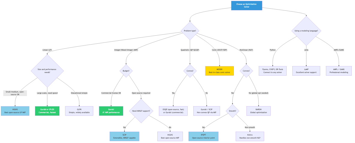
Solver Selection Guide
| Problem Type | Recommended Solver(s) |
|---|---|
| LP (small-medium) | HiGHS, Gurobi, CPLEX |
| LP (large sparse) | Gurobi (barrier), MOSEK |
| MIP | Gurobi, CPLEX, SCIP (open-source) |
| SOCP | MOSEK, Gurobi, ECOS |
| SDP | MOSEK, SCS (large-scale) |
| QP | OSQP (real-time), Gurobi |
| NLP | IPOPT, SNOPT, Knitro |
| Global MINLP | BARON, SCIP, Couenne |
| CP / Scheduling | CP-SAT (OR-Tools), CP Optimizer (CPLEX) |
| Large-scale conic | SCS, COSMO |
Connections
- LP solver internals: simplex and IPM (→
01-linear-programming.md). - MIP solver techniques: branch and cut (→
02-integer-programming.md). - Conic solver theory (→
05-conic-programming.md). - NLP solver methods (→
06-nonlinear-programming.md). - Combinatorial solvers: CP, SAT (→
07-combinatorial-optimization.md).