Language Models

Overview

A language model assigns probabilities to sequences of tokens. It captures the statistical structure of language and serves as the foundation for generation, classification, and understanding tasks. The field has progressed from count-based n-gram models to massive neural models exhibiting emergent capabilities.

N-gram Language Models

An n-gram model estimates the probability of a word given the previous n-1 words using maximum likelihood estimation from counts.

P(w_t | w_{t-n+1}, ..., w_{t-1}) = count(w_{t-n+1}...w_t) / count(w_{t-n+1}...w_{t-1})

Sparsity and Smoothing

Most n-grams never appear in training data, yielding zero probabilities. Smoothing redistributes probability mass to unseen events.

| Method | Idea | |---|---| | Laplace (add-1) | Add 1 to all counts; simple but over-smooths | | Add-k | Add k < 1; slightly better | | Backoff | Fall back to (n-1)-gram when n-gram count is zero | | Interpolation | Weighted mixture of unigram through n-gram estimates | | Kneser-Ney | Discount fixed amount from each count; distribute mass based on continuation probability |

Kneser-Ney Smoothing

The key insight: a word's backoff probability should reflect how many different contexts it appears in (continuation count), not its raw frequency.

"Francisco" is frequent but almost always follows "San" -- low continuation count
"the" appears in many contexts -- high continuation count
Modified Kneser-Ney (with multiple discount values) is the gold standard for n-gram LMs

Perplexity

The standard intrinsic evaluation metric for language models.

PP(W) = P(w_1, w_2, ..., w_N)^{-1/N}
      = exp(- (1/N) sum log P(w_t | context))

Lower perplexity = better model (assigns higher probability to test data)
Equivalent to the exponential of cross-entropy
A perplexity of k means the model is as uncertain as choosing uniformly among k options
Only comparable between models using the same vocabulary/tokenization

Neural Language Models

Feed-forward Neural LM (Bengio et al., 2003)

Fixed context window of n-1 words, each mapped to an embedding
Concatenated embeddings passed through hidden layers to predict next word
First to show that learned embeddings + neural prediction outperform n-grams
Limited by fixed context window

Recurrent Neural LMs

RNNs process sequences of arbitrary length with a hidden state
LSTMs and GRUs solve the vanishing gradient problem
Theoretically unlimited context but practically limited to ~200 tokens
Trained with truncated backpropagation through time

Transformer-based LMs

Transformer Architecture with Encoder, Decoder, and Attention

Transformers use self-attention to model long-range dependencies in parallel. Three main architectures define modern LMs.

Autoregressive Models (Decoder-only)

Generate text left-to-right; each token attends only to previous tokens (causal masking).

Architecture: Stack of transformer decoder blocks with causal self-attention.

Training objective: Next-token prediction.

L = -sum_t log P(x_t | x_1, ..., x_{t-1})

Examples: GPT-2, GPT-3, GPT-4, LLaMA, Mistral, Claude

Properties:

Natural fit for text generation
In-context learning emerges at scale
Scale well with more parameters and data
Dominate current LLM landscape

Masked Language Models (Encoder-only)

Bidirectional: each token attends to all other tokens. Not autoregressive.

Training objective: Mask 15% of tokens; predict the masked tokens from context.

L = -sum_{t in masked} log P(x_t | x_{\masked})

Examples: BERT, RoBERTa, ALBERT, DeBERTa

Properties:

Bidirectional context produces strong representations for understanding tasks
Not naturally suited for generation
Fine-tuned for classification, NER, QA, etc.
RoBERTa improvements: more data, longer training, dynamic masking, no NSP

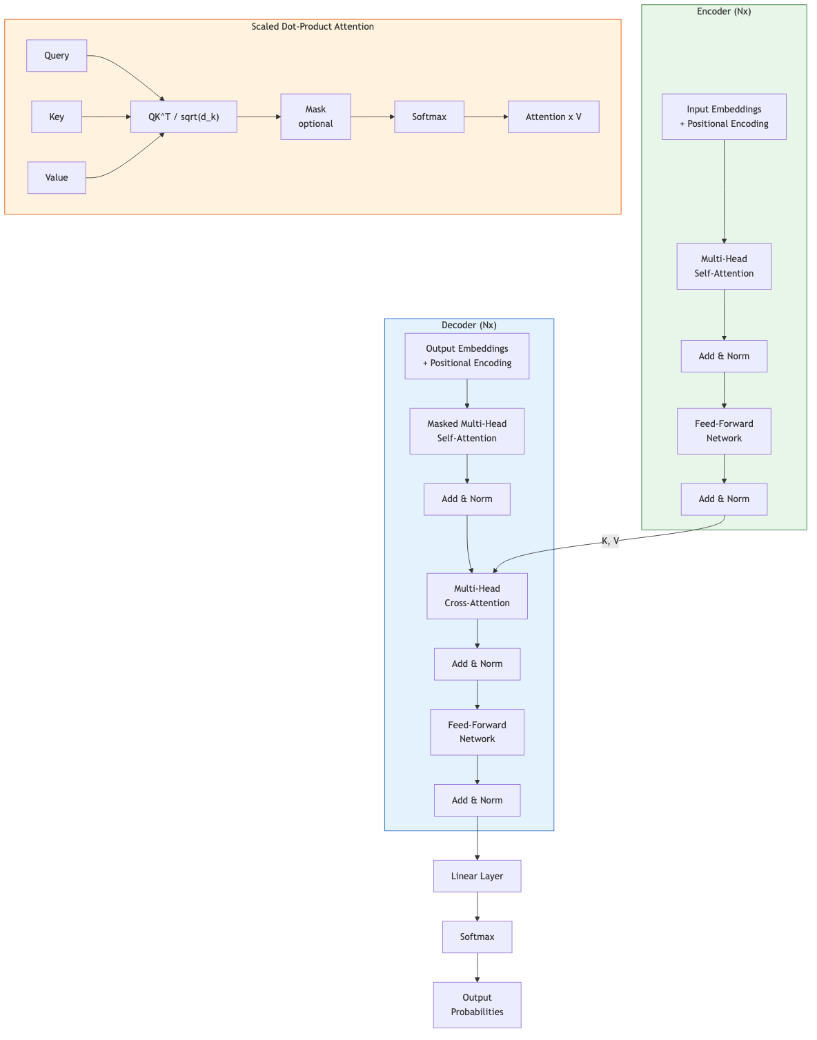
Encoder-Decoder Models

Encoder processes input bidirectionally; decoder generates output autoregressively, attending to encoder representations via cross-attention.

Training objective: Typically span corruption (T5) -- mask spans of text, generate the masked spans.

Examples: T5, BART, mT5, Flan-T5

Properties:

Natural for sequence-to-sequence tasks (translation, summarization)
T5 frames all tasks as text-to-text
BART uses denoising autoencoder pretraining (deletion, infilling, shuffling, masking)

Scaling Laws

Kaplan et al. (2020) and Hoffmann et al. (2022, "Chinchilla") established power-law relationships.

L(N, D) ~ a/N^alpha + b/D^beta + c

Where N = parameters, D = data tokens, L = loss.

Key findings:

Loss decreases as a power law with both model size and data size
Chinchilla scaling: optimal training uses roughly 20 tokens per parameter
GPT-3 (175B params, 300B tokens) was undertrained by Chinchilla standards
LLaMA showed strong performance by training smaller models on much more data

Compute-Optimal Training

| Model | Parameters | Training Tokens | Ratio | |---|---|---|---| | Chinchilla | 70B | 1.4T | 20:1 | | LLaMA | 7-65B | 1-1.4T | 20-200:1 | | LLaMA 2 | 7-70B | 2T | 29-286:1 |

The trend has shifted toward overtrained smaller models for cheaper inference.

Emergent Abilities

Capabilities that appear suddenly at a certain scale, absent in smaller models.

Chain-of-thought reasoning: step-by-step problem solving
Arithmetic: multi-digit addition/multiplication
Code generation: writing functional programs
Multilingual transfer: performance on languages with little training data
Debate exists on whether emergence is real or an artifact of metric choice (Wei et al. vs Schaeffer et al.)

In-Context Learning (ICL)

The ability to perform tasks by conditioning on examples in the prompt, without gradient updates.

Zero-shot: Task description only, no examples. Few-shot: Task description plus k input-output examples.

Translate English to French:
sea otter => loutre de mer
cheese => fromage
hello =>

Properties:

Performance improves with more examples (up to a point)
Sensitive to example ordering and formatting
May perform pattern matching rather than true learning
Theoretical explanations include implicit Bayesian inference, mesa-optimization, and in-context gradient descent

Training Infrastructure

Modern LMs require distributed training across many accelerators.

| Technique | What It Parallelizes | |---|---| | Data parallelism | Replicate model, split data across devices | | Tensor parallelism | Split individual layers across devices | | Pipeline parallelism | Split layers across devices in stages | | Expert parallelism | Route tokens to different experts (MoE) | | ZeRO (DeepSpeed) | Shard optimizer states, gradients, parameters | | FSDP (PyTorch) | Fully sharded data parallelism |

Mixed-precision training (FP16/BF16 with FP32 master weights) and gradient checkpointing reduce memory.

Key Takeaways

N-gram models with Kneser-Ney smoothing were the standard for decades and remain useful baselines
Perplexity measures how well a model predicts held-out text; lower is better
The three transformer LM architectures (autoregressive, masked, encoder-decoder) serve different purposes
Scaling laws predict that loss decreases as a power law with compute, data, and parameters
Emergent abilities and in-context learning make large autoregressive models qualitatively different from smaller ones
Compute-optimal training balances model size against data quantity