Error Analysis

Numerical computation introduces errors at every step. Understanding error sources, propagation, and stability is essential for writing reliable scientific software.

Floating-Point Arithmetic

IEEE 754 Representation

A floating-point number is stored as:

(-1)^s × m × 2^e

| Format | Sign | Exponent | Mantissa | Total bits | Decimal digits | |---|---|---|---|---|---| | Single (f32) | 1 | 8 | 23 | 32 | ~7 | | Double (f64) | 1 | 11 | 52 | 64 | ~15-16 |

The mantissa has an implicit leading 1 (normalized form): m = 1.b₁b₂...bₚ.

Special Values

• +0, -0: Signed zeros (equal in comparison but distinguishable)
• +∞, -∞: Result of overflow or division by zero
• NaN (Not a Number): Result of 0/0, ∞-∞, √(-1). NaN ≠ NaN.
• Subnormal numbers: Very small numbers near zero (gradual underflow)

Machine Epsilon

Machine epsilon ε_mach is the smallest number such that fl(1 + ε) > 1.

f32: ε_mach ≈ 1.19 × 10⁻⁷
f64: ε_mach ≈ 2.22 × 10⁻¹⁶

It represents the relative precision of the floating-point system. For any real number x representable in the range:

fl(x) = x(1 + δ)   where |δ| ≤ ε_mach/2  (round-to-nearest)

Representable Numbers

Floating-point numbers are not uniformly spaced. They are densely packed near zero and sparse for large values.

Between 1 and 2: spacing is ε_mach. Between 2 and 4: spacing is 2ε_mach. Between 2ᵏ and 2ᵏ⁺¹: spacing is 2ᵏ · ε_mach.

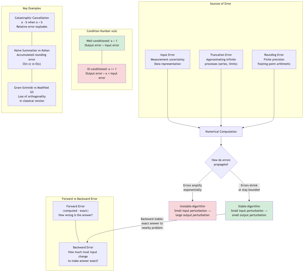
Types of Errors

Rounding Errors

Arise from representing real numbers in finite precision.

Example: 1/3 = 0.333... cannot be exactly represented.

Example: 0.1 in binary is 0.0001100110011... (repeating), so 0.1 + 0.2 ≠ 0.3 in floating-point.

// Floating-point rounding demonstration
a ← 0.1 + 0.2
PRINT a              // outputs 0.30000000000000004
PRINT (a = 0.3)      // outputs false

Truncation Errors

Arise from approximating infinite processes with finite ones.

Example: Taylor series truncated after n terms:

sin(x) ≈ x - x³/3! + x⁵/5! - ... ± xⁿ/n!

The truncation error is bounded by the next term (for alternating series).

Example: Numerical derivative:

f'(x) ≈ (f(x+h) - f(x)) / h

Truncation error = O(h) from Taylor expansion. Smaller h → smaller truncation error but larger rounding error.

Discretization Errors

Arise from replacing continuous domains with discrete ones (grids, meshes). A form of truncation error for PDEs.

Catastrophic Cancellation

When subtracting two nearly equal numbers, significant digits are lost.

Example: Compute √(x² + 1) - x for large x.

x = 10⁸:
√(10¹⁶ + 1) = 100000000.000000005...
100000000.000000005 - 100000000 = 5 × 10⁻⁹

But in f64: both round to the same value → result = 0 (completely wrong!)

Fix: Rationalize: √(x²+1) - x = 1/(√(x²+1) + x). For x = 10⁸: 1/(2×10⁸) = 5×10⁻⁹. ✓

Common Cancellation Scenarios

Quadratic formula: x = (-b ± √(b²-4ac))/(2a). When b² ≫ 4ac, one root suffers cancellation.

Fix: Compute the larger root directly, then use x₁x₂ = c/a for the other.

Variance: Computing Σ(xᵢ - x̄)² directly can cancel. Use the two-pass formula or Welford's online algorithm.

Example: Dataset [10000000, 10000001, 10000002]. Naive Σxᵢ² - n·x̄² suffers massive cancellation.

Condition Number

The condition number of a problem measures its sensitivity to input perturbations.

For a Function

κ = |x f'(x) / f(x)|

The relative change in output per relative change in input.

Example: f(x) = √x. κ = |x · 1/(2√x) / √x| = 1/2. Well-conditioned.

Example: f(x) = ln(x) near x = 1. κ = |x · (1/x) / ln(x)| = |1/ln(x)|. As x → 1, κ → ∞. Ill-conditioned near x = 1.

For Linear Systems

The condition number of matrix A:

κ(A) = ‖A‖ · ‖A⁻¹‖

Using the 2-norm: κ₂(A) = σ_max / σ_min (ratio of largest to smallest singular value).

Interpretation: When solving Ax = b, a relative perturbation δb/b in the right-hand side can cause a relative change of up to κ(A) · δb/b in the solution.

‖δx‖/‖x‖ ≤ κ(A) · ‖δb‖/‖b‖

| κ(A) | Interpretation | |---|---| | ~1 | Well-conditioned | | ~10⁶ | Lose ~6 decimal digits | | ~10¹⁶ | Nearly singular (for f64) |

Rule of thumb: With f64 (16 digits), you can trust about 16 - log₁₀(κ) digits of the solution.

Numerical Stability

An algorithm is numerically stable if it produces results close to the exact answer for the exact input (or equivalently, produces the exact answer for a slightly perturbed input — backward stability).

Forward Error

forward error = |computed result - exact result|

Backward Error

backward error = smallest perturbation to input that makes the computed result exact

An algorithm is backward stable if the backward error is small (comparable to rounding error in the input).

Examples

Gaussian elimination with partial pivoting: Backward stable. The computed solution x̂ exactly solves (A + δA)x̂ = b where ‖δA‖ is small.

Gaussian elimination without pivoting: Unstable. Can fail spectacularly even for well-conditioned problems.

Gram-Schmidt (classical): Numerically unstable. Modified Gram-Schmidt is better. Householder QR is backward stable.

Computing eigenvalues via characteristic polynomial roots: Unstable. QR algorithm is backward stable.

Error Propagation

For Arithmetic Operations

| Operation | Absolute Error | Relative Error | |---|---|---| | x + y | δx + δy | (δx + δy)/(x + y) | | x - y | δx + δy | (δx + δy)/(x - y) — huge if x ≈ y! | | x × y | |y|δx + |x|δy | δx/x + δy/y | | x / y | (|y|δx + |x|δy)/y² | δx/x + δy/y |

Subtraction is dangerous when operands are nearly equal (cancellation).

Forward Error Analysis

Track errors through each operation step by step. Tedious but exact.

Backward Error Analysis

Pioneered by Wilkinson. Instead of tracking forward error, show that the result is the exact answer to a nearby problem. More elegant and practical for complex algorithms.

Practical Guidelines

1. Avoid subtracting nearly equal quantities. Reformulate the expression.
2. Add small numbers first when summing many terms (Kahan summation for better accuracy).
3. Use stable algorithms: Partial pivoting in LU, Householder QR, divide-and-conquer SVD.
4. Check condition numbers before solving linear systems.
5. Use appropriate precision: f64 for most work. f128 or arbitrary precision for special cases.
6. Validate numerics: Compare with analytical solutions, vary parameters, check residuals.
7. Beware of iterative algorithms: Check convergence, don't iterate too long (error may grow).

Kahan Summation

Compensates for floating-point errors when summing many values:

FUNCTION KAHAN_SUM(values)
    sum ← 0.0
    c ← 0.0  // compensation
    FOR EACH v IN values DO
        y ← v - c
        t ← sum + y
        c ← (t - sum) - y  // recovers lost low-order bits
        sum ← t
    RETURN sum

Reduces error from O(nε) to O(ε), independent of n.

Applications in CS

• Scientific computing: Every numerical simulation must account for floating-point errors. Condition numbers determine feasibility.
• Machine learning: Gradient computation, loss functions (log-sum-exp trick for numerical stability), mixed-precision training (f16/bf16 + f32).
• Computer graphics: Ray-object intersection at grazing angles, thin triangles, degenerate geometry — all need careful numerics.
• Cryptography: Constant-time arithmetic to avoid timing side channels. Exact integer arithmetic for RSA.
• Financial computing: Decimal arithmetic (not binary float) for currency. Or fixed-point with integer cents.
• Computational geometry: Exact predicates (Shewchuk's orientation/incircle tests) to avoid topological errors from rounding.
• Database systems: Decimal types for financial data. Floating-point aggregation order matters.