Root Finding

Root finding algorithms solve f(x) = 0. They are fundamental building blocks — used in optimization, equation solving, inverse function evaluation, and implicit surface rendering.

Root-Finding Methods Comparison

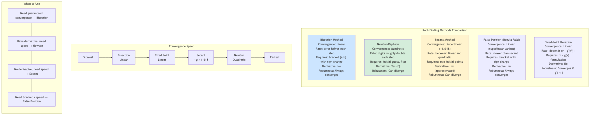
Bisection Method

The simplest root-finding method, based on the Intermediate Value Theorem.

Algorithm

Given f continuous on [a, b] with f(a) · f(b) < 0 (sign change):

while |b - a| > tolerance:
    c = (a + b) / 2
    if f(c) = 0: return c
    if f(a) · f(c) < 0: b = c
    else: a = c
return (a + b) / 2

Properties

Convergence: Guaranteed (if initial bracket is valid)
Rate: Linear. Error halves each iteration: eₙ₊₁ = eₙ/2
Iterations needed: log₂((b-a)/ε) for tolerance ε
Robustness: Very robust. No derivative needed. Never fails (within bracket).

FUNCTION BISECTION(f, a, b, tol)
    ASSERT f(a) * f(b) < 0  // "No sign change"
    WHILE |b - a| > tol DO
        c ← (a + b) / 2
        IF f(a) * f(c) ≤ 0 THEN b ← c
        ELSE a ← c
    RETURN (a + b) / 2

Newton's Method (Newton-Raphson)

Uses the tangent line to approximate the root.

Algorithm

x_{n+1} = xₙ - f(xₙ) / f'(xₙ)

Derived from: the tangent line at xₙ is y = f(xₙ) + f'(xₙ)(x - xₙ). Set y = 0 and solve for x.

Convergence

Quadratic convergence near simple roots: eₙ₊₁ ≈ C · eₙ²
The number of correct digits roughly doubles each iteration
Requires a good initial guess (may diverge otherwise)
Fails when f'(xₙ) = 0 (horizontal tangent)

Convergence Analysis

Near a simple root r, Taylor expansion gives:

eₙ₊₁ = -f''(r)/(2f'(r)) · eₙ² + O(eₙ³)

For multiple roots (f(r) = f'(r) = 0), convergence degrades to linear. Modified Newton: x_{n+1} = xₙ - m · f(xₙ)/f'(xₙ) with multiplicity m restores quadratic convergence.

Practical Considerations

Can oscillate or diverge with poor initial guess
May cycle (e.g., f(x) = x³ - 2x + 2 from x₀ = 0)
Combine with bisection as safeguard (Brent's method)

FUNCTION NEWTON(f, df, x, tol, max_iter)
    FOR i ← 1 TO max_iter DO
        fx ← f(x)
        IF |fx| < tol THEN RETURN x
        x ← x - fx / df(x)
    RETURN x

Secant Method

Like Newton's method but approximates f'(x) using a secant line (no derivative needed).

Algorithm

x_{n+1} = xₙ - f(xₙ) · (xₙ - xₙ₋₁) / (f(xₙ) - f(xₙ₋₁))

Properties

No derivative required (only function evaluations)
Superlinear convergence: Order ≈ 1.618 (golden ratio φ): eₙ₊₁ ≈ C · eₙ^φ
Needs two initial points
Not guaranteed to converge (no bracketing)

Fixed-Point Iteration

Rewrite f(x) = 0 as x = g(x) and iterate:

x_{n+1} = g(xₙ)

Convergence Condition

Converges if |g'(x)| < 1 near the fixed point (contraction mapping theorem).

|g'(r)| < 1: convergent
|g'(r)| > 1: divergent
Smaller |g'(r)| → faster convergence

Example: Solve x = cos(x). Iterate xₙ₊₁ = cos(xₙ). Converges to x ≈ 0.7391 (the Dottie number).

Newton's method is a special case: g(x) = x - f(x)/f'(x), which has g'(r) = 0 for simple roots (hence quadratic convergence).

Muller's Method

Uses a quadratic through three points instead of a line. Can find complex roots even with real starting points.

Fit parabola through (xₙ₋₂, fₙ₋₂), (xₙ₋₁, fₙ₋₁), (xₙ, fₙ)
x_{n+1} = root of the parabola closest to xₙ

Convergence order: ≈ 1.84. Superlinear, between secant and Newton.

Brent's Method

The gold standard for robust root finding. Combines bisection, secant, and inverse quadratic interpolation.

Strategy

Maintains a bracket [a, b] at all times (guaranteed convergence)
Uses secant or inverse quadratic interpolation when they make progress
Falls back to bisection when fast methods fail or would leave the bracket

Properties

Guaranteed convergence (like bisection)
Superlinear convergence in practice (like secant/Newton)
No derivative needed
Used in most numerical libraries (e.g., scipy.optimize.brentq)

Convergence: At least as fast as bisection, often much faster. Worst case: same as bisection.

Polynomial Root Finding

Companion Matrix Method

The roots of p(x) = xⁿ + aₙ₋₁xⁿ⁻¹ + ... + a₁x + a₀ are the eigenvalues of the companion matrix:

C = [0    0    ...  0   -a₀  ]
    [1    0    ...  0   -a₁  ]
    [0    1    ...  0   -a₂  ]
    [⋮    ⋮     ⋱   ⋮    ⋮   ]
    [0    0    ...  1  -aₙ₋₁ ]

Reduces polynomial root finding to eigenvalue computation (QR algorithm). Numerically stable. Used by MATLAB's roots and numpy's numpy.roots.

Durand-Kerner Method

Simultaneous iteration for all roots:

z_i^{(k+1)} = z_i^{(k)} - p(z_i^{(k)}) / Πⱼ≠ᵢ (z_i^{(k)} - z_j^{(k)})

All roots are updated simultaneously. Converges quadratically with good initial guesses.

Aberth Method

Similar to Durand-Kerner but with better convergence (cubic). Used in MPSolve for high-precision polynomial root finding.

Systems of Nonlinear Equations

Multivariate Newton's Method

Solve F(x) = 0 where F: ℝⁿ → ℝⁿ:

x_{n+1} = xₙ - J(xₙ)⁻¹ F(xₙ)

where J is the Jacobian matrix. In practice, solve the linear system J(xₙ) · δx = -F(xₙ) instead of inverting J.

Quadratic convergence near a simple root (non-singular Jacobian).

Cost: One Jacobian evaluation + one linear system solve per iteration.

Quasi-Newton Methods

Approximate the Jacobian to avoid expensive evaluations:

Broyden's method: Rank-1 updates to an approximate Jacobian. Superlinear convergence.

| Method | Order | Function evals per step | Derivative needed | |---|---|---|---| | Bisection | 1 (linear) | 1 | No | | Fixed-point iteration | 1 (linear) | 1 | No | | Secant | ~1.618 | 1 | No | | Muller | ~1.84 | 1 | No | | Newton | 2 (quadratic) | 1 + derivative | Yes | | Halley | 3 (cubic) | 1 + 2 derivatives | Yes |

Efficiency index = p^(1/d) where p is convergence order and d is function evaluations per step. Newton: 2^(1/2) ≈ 1.41. Secant: 1.618^(1/1) = 1.618. Secant wins on efficiency!

Applications in CS

Optimization: Finding critical points (f'(x) = 0) via Newton on the gradient.
Computer graphics: Ray-surface intersection for implicit surfaces uses Newton/bisection.
Finance: Implied volatility computation (Black-Scholes inversion) uses Brent's method.
Signal processing: Finding poles and zeros of transfer functions.
Game physics: Collision detection (time-of-impact) uses root finding.
Machine learning: Logistic regression (IRLS is Newton's method). Finding optimal hyperparameters.
Compiler optimization: Fixed-point iteration for dataflow analysis.
Network protocols: TCP congestion control algorithms implicitly solve equations.