Static Analysis Foundations

Fundamental Limits and Tradeoffs

Rice's Theorem and Undecidability

Rice's theorem states that every non-trivial semantic property of programs is undecidable. A property is non-trivial if some programs satisfy it and some do not. Consequently, no algorithm can decide, for all programs, whether a given semantic property holds. This forces static analysis to approximate: every practical analyzer must sacrifice either soundness (reporting all true facts) or completeness (reporting only true facts), or both.

Soundness vs. Completeness

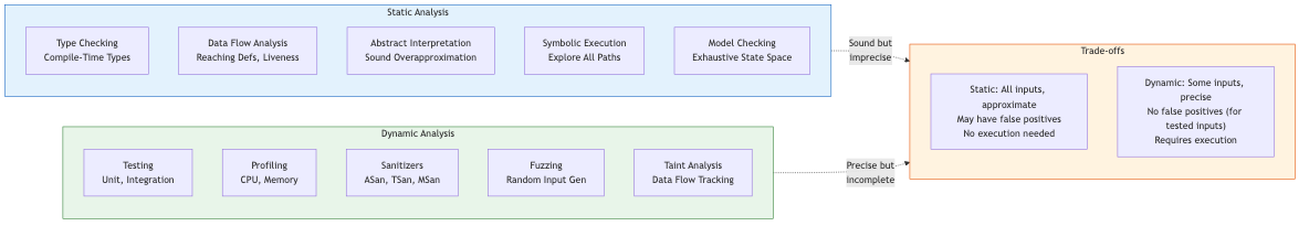
• Sound analysis: overapproximates program behavior. If the analysis says "property P does not hold," then P genuinely does not hold. Sound analyses may produce false positives (spurious warnings) but never miss true violations. Compilers and safety-critical verification demand soundness.
• Complete analysis: underapproximates program behavior. If the analysis reports a violation, that violation is genuine. Complete analyses may produce false negatives (missed bugs) but every reported issue is real. Bug-finding tools (e.g., fuzzing, bounded model checking) often aim here.
• Pragmatic analyzers: many industrial tools (Coverity, Infer in some modes) are neither fully sound nor complete but aim for a useful balance.

May vs. Must Analysis

• May analysis answers: "Can this happen on some execution path?" Overapproximates reachable states. Used for safety properties — if a may analysis says a variable may be uninitialized, the compiler inserts a warning.
• Must analysis answers: "Does this happen on all execution paths?" Underapproximates reachable states. Used for optimization — if a must analysis says an expression is always available, the optimizer can eliminate redundant computation.

The duality: may analysis of property P is equivalent to must analysis of ¬P over reversed control flow in many frameworks.

Control Flow Analysis

Control Flow Graphs (CFGs)

A CFG represents the flow of control within a procedure. Nodes are basic blocks (maximal sequences of straight-line instructions), edges represent possible transfers of control (branches, jumps, fall-through). Construction is straightforward for structured languages; unstructured gotos and exceptions require care.

Dominance: Node A dominates node B if every path from the entry to B passes through A. The immediate dominator idom(B) is the closest strict dominator. The dominator tree encodes the dominance relation efficiently, computable in nearly-linear time via the Lengauer-Tarjan algorithm.

Post-dominance: Dual notion on reversed CFG. Node A post-dominates B if every path from B to exit passes through A.

Control dependence: Node B is control-dependent on node A if A has two successors, one that must pass through B and one that can avoid B. This drives program slicing and SSA placement.

Loop Analysis

Natural loops: identified via back edges (edges to dominators) in the dominator tree. The loop body consists of all nodes from which the loop header is reachable without traversing the back edge target. Loop nesting forests organize loops hierarchically, essential for optimizations like loop-invariant code motion.

Data Flow Analysis

The Monotone Framework

Data flow analysis computes facts at each program point by propagating information along CFG edges. The monotone framework formalizes this.

Components:

1. A complete lattice (L, ⊑) with finite height (ascending chain condition)
2. A transfer function f_n : L → L for each node n, monotone (x ⊑ y ⟹ f(x) ⊑ f(y))
3. A merge operator (⊔ for may, ⊓ for must) at join points
4. An initial value for the entry/exit node

Fixed-point theorem (Tarski): Because L has finite height and transfer functions are monotone, iterative application converges to the least fixed point (for may/forward) or greatest fixed point (for must/backward).

Classical Analyses

Reaching Definitions

• Direction: Forward
• Lattice: Sets of definitions (gen/kill), ordered by ⊆
• Merge: Union (may analysis)
• Transfer: OUT[B] = (IN[B] \ kill[B]) ∪ gen[B]
• Application: Detecting uninitialized variables, building def-use chains

A definition d: x = ... at point p reaches point q if there exists a path from p to q with no intervening redefinition of x.

Live Variables

• Direction: Backward
• Lattice: Sets of variables, ordered by ⊆
• Merge: Union (may analysis)
• Transfer: IN[B] = (OUT[B] \ def[B]) ∪ use[B]
• Application: Register allocation, dead code elimination

A variable v is live at point p if there exists a path from p to a use of v with no intervening definition.

Available Expressions

• Direction: Forward
• Lattice: Sets of expressions, ordered by ⊇ (note: reversed!)
• Merge: Intersection (must analysis)
• Transfer: OUT[B] = (IN[B] \ kill[B]) ∪ gen[B]
• Application: Common subexpression elimination

An expression e is available at point p if on every path from entry to p, e is computed and none of its operands are subsequently redefined.

Very Busy Expressions

• Direction: Backward
• Lattice: Sets of expressions, ordered by ⊇
• Merge: Intersection (must analysis)
• Transfer: IN[B] = (OUT[B] \ kill[B]) ∪ gen[B]
• Application: Code hoisting

An expression is very busy at point p if on every path from p it is evaluated before any of its operands are redefined.

Gen/Kill Framework

Many bit-vector analyses fit the gen/kill pattern: OUT = (IN \ kill) ∪ gen. Transfer functions in this form are always monotone and distributive (f(x ⊔ y) = f(x) ⊔ f(y)), meaning the MOP (meet-over-all-paths) solution equals the MFP (maximal fixed point) solution — no precision is lost by merge.

For non-distributive analyses (e.g., constant propagation), MFP may be strictly less precise than MOP. Consider: two paths assign x=2 and x=3; merging yields x=⊤ (not constant), but on each individual path, x is constant.

Worklist Algorithms

Iterative Round-Robin

The simplest approach: repeatedly iterate over all nodes in some order until no values change. Convergence is guaranteed but potentially slow: O(h × n × k) where h is lattice height, n is node count, k is per-node cost.

Worklist-Based Iteration

Maintain a worklist (set/queue) of nodes whose inputs have changed. Process a node, compute its new output; if changed, add successors to the worklist. More efficient: only re-processes nodes affected by changes.

Ordering heuristics:

• Reverse postorder (RPO): Process nodes in topological-ish order. For acyclic graphs, single pass suffices. For loops, inner loops converge before outer.
• Reverse postorder on the reverse CFG: Optimal for backward analyses.
• Priority worklist: Use RPO numbering as priority; process lowest-numbered node first.

Convergence Speed

For bit-vector frameworks with RPO ordering: convergence in d+3 passes where d is the loop nesting depth. For general monotone frameworks: bounded by lattice height × number of nodes, but practical convergence is much faster with good ordering.

SSA Form and Sparse Analysis

Static Single Assignment

SSA form requires every variable to have exactly one definition point. At join points, φ-functions merge values: x₃ = φ(x₁, x₂). SSA is constructed via dominance frontiers (Cytron et al.) or by the simpler but equivalent approach of iterated dominance frontiers.

Benefits for analysis: SSA makes def-use chains explicit, converting dense data flow problems into sparse ones. Instead of propagating over every program point, analysis follows SSA edges directly.

Sparse Analysis

Traditional data flow analysis computes facts at every program point. Sparse analysis computes facts only where relevant definitions/uses occur, using SSA def-use chains. This can yield orders-of-magnitude speedup for large programs while computing identical results.

Sparse conditional constant propagation (Wegman-Zadeck): Combines constant propagation with unreachable code elimination. Uses two worklists: one for SSA edges (value propagation) and one for CFG edges (reachability). Only processes reachable code and only propagates along SSA edges — both sparse and flow-sensitive.

Type-Based and Constraint-Based Analysis

Type Systems as Static Analysis

Type checking is a form of static analysis. Hindley-Milner type inference solves constraint systems to assign types. Richer type systems (refinement types, dependent types, linear types) verify deeper properties but increase annotation burden or analysis complexity.

Set Constraints

Many analyses reduce to solving set constraints. For example, control flow analysis in higher-order languages (0-CFA, k-CFA) generates inclusion constraints among sets of possible values. Cubic-time algorithms (Aiken, Heintze) solve these constraints.

0-CFA (zeroth-order control flow analysis): For each expression, compute the set of lambda terms it might evaluate to. Generates constraints: if f might be λx.e and f is applied to argument a, then the values of a flow into x and the values of e flow to the call site. Fixed point of these constraints gives a sound approximation.

Convergence and Precision Hierarchy

Precision of static analyses can be organized along several dimensions:

| Dimension | Less precise | More precise | |-----------|-------------|--------------| | Flow sensitivity | Flow-insensitive | Flow-sensitive | | Path sensitivity | Path-insensitive | Path-sensitive | | Context sensitivity | Context-insensitive | Context-sensitive | | Field sensitivity | Field-insensitive | Field-sensitive | | Object sensitivity | Allocation-site | Recency / type-sensitive |

Each increase in precision generally increases cost. Flow-insensitive analysis ignores control flow order (single abstract state for entire program). Flow-sensitive analysis maintains per-program-point abstract states. Path-sensitive analysis distinguishes states based on branch conditions (exponential blowup). Context-sensitive analysis distinguishes different calling contexts (see interprocedural analysis).

Practical Considerations

Scalability

Industrial codebases have millions of lines of code. Scalable analysis requires:

• Efficient representations: BDDs, sparse bitvectors, shared data structures
• Demand-driven evaluation: Compute only what is queried
• Modular analysis: Analyze functions/modules independently, compose summaries
• Parallelism: Concurrent fixed-point iteration on independent SCCs of the call graph

Soundness in Practice

Few industrial tools are truly sound. Sources of unsoundness include: reflection, dynamic loading, native code, inline assembly, concurrency, unmodeled library behavior, and deliberate unsound choices for reduced false positives. Tools like Astrée achieve soundness for restricted language subsets in safety-critical domains.