Discrete-Event Simulation
Core Concepts
In DES, the system state changes only at discrete points called events. Between events, nothing changes. The simulation clock jumps from one event to the next, making DES efficient for systems with sparse activity relative to wall-clock time.
Components
- Entities — Objects that flow through the system (customers, packets, jobs)
- Resources — Shared capacity that entities compete for (servers, machines, lanes)
- Events — Instantaneous state transitions (arrival, service start, departure)
- State variables — Quantities tracked over time (queue length, server status)
- Statistical accumulators — Collect output metrics (average wait, throughput)
Event Scheduling Approach
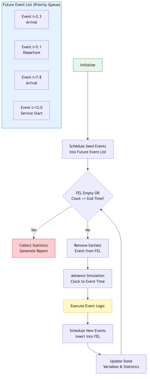
The simulation maintains a Future Event List (FEL) — a time-ordered collection of scheduled events. The main loop:
initialize FEL with seed events
while FEL is not empty and clock < end_time:
    remove earliest event from FEL
    advance clock to event time
    execute event logic (may schedule new events)
    update statistics
ENUMERATION EventType ← {ARRIVAL, DEPARTURE}

STRUCTURE Event
    time: real
    event_type: EventType

STRUCTURE Simulation
    clock: real
    fel: min-priority queue of Event (ordered by time)
    server_busy: boolean
    queue_len: integer
    total_wait: real
    served: integer

PROCEDURE RUN(sim, end_time)
    WHILE sim.fel IS NOT empty DO
        event ← EXTRACT_MIN(sim.fel)
        IF event.time > end_time THEN BREAK
        sim.clock ← event.time
        IF event.event_type = ARRIVAL THEN
            HANDLE_ARRIVAL(sim)
        ELSE IF event.event_type = DEPARTURE THEN
            HANDLE_DEPARTURE(sim)

PROCEDURE HANDLE_ARRIVAL(sim)
    // Schedule next arrival
    interarrival ← EXPONENTIAL_RANDOM(rate ← 1.0)
    INSERT(sim.fel, Event(time ← sim.clock + interarrival, type ← ARRIVAL))
    IF sim.server_busy THEN
        sim.queue_len ← sim.queue_len + 1
    ELSE
        sim.server_busy ← TRUE
        service ← EXPONENTIAL_RANDOM(rate ← 1.5)
        INSERT(sim.fel, Event(time ← sim.clock + service, type ← DEPARTURE))

PROCEDURE HANDLE_DEPARTURE(sim)
    sim.served ← sim.served + 1
    IF sim.queue_len > 0 THEN
        sim.queue_len ← sim.queue_len - 1
        service ← EXPONENTIAL_RANDOM(rate ← 1.5)
        INSERT(sim.fel, Event(time ← sim.clock + service, type ← DEPARTURE))
    ELSE
        sim.server_busy ← FALSE

PROCEDURE EXPONENTIAL_RANDOM(rate) → real
    // -ln(1 - U) / rate, where U ~ Uniform(0,1)
    RETURN -LN(1.0 - RANDOM()) / rate
Process Interaction Approach
Instead of writing event handlers, model each entity as a process (coroutine) that describes its entire lifecycle: arrive, seize resource, delay, release resource, depart.
process Customer:
    enter system
    if server available:
        seize server
    else:
        wait in queue
    delay(service_time)
    release server
    collect statistics
    depart
Process interaction is more natural for complex workflows but requires coroutine or thread support.
Simulation Clock and Time Advancement
Next-event time advance: clock jumps to the time of the next imminent event. No computation occurs between events.
Fixed-increment time advance: clock advances by Δt each step, checking for events within each interval. Simpler but wastes cycles when events are sparse.
DES almost always uses next-event advancement. The FEL is typically a binary heap (priority queue) giving O(log n) insert and O(log n) extract-min.
Random Variate Generation
Inverse Transform Method
If F is the CDF of the desired distribution and U ~ Uniform(0,1):
X = F⁻¹(U)
Works for distributions with closed-form inverse CDFs:
- Exponential: X = -ln(1-U) / λ
- Uniform(a,b): X = a + (b-a)U
- Weibull: X = β(-ln(1-U))^(1/α)
Acceptance-Rejection Method
For distributions without tractable inverse CDFs (e.g., Beta, Gamma):
- Find an envelope distribution g(x) such that f(x) ≤ c·g(x) for all x
- Generate Y from g, U from Uniform(0,1)
- If U ≤ f(Y) / (c·g(Y)), accept X = Y; else reject and repeat
Efficiency = 1/c, so tight envelopes are crucial.
Special Methods
- Box-Muller for Normal: two uniforms produce two independent normals
- Convolution for Erlang-k: sum of k exponentials
- Composition for mixture distributions
Input Modeling
Distribution Fitting Workflow
- Collect real-world data (interarrival times, service durations)
- Plot histogram, compute summary statistics
- Hypothesize candidate distributions
- Estimate parameters (MLE, method of moments)
- Goodness-of-fit test (Chi-square, K-S, Anderson-Darling)
- Select best fit; if none adequate, use empirical distribution
Common Distributions in DES
| Distribution | Typical Use |
|---|---|
| Exponential | Interarrival times (memoryless) |
| Normal/LogNormal | Processing times |
| Uniform | Bounded uncertainty |
| Triangular | Expert-estimated durations |
| Poisson | Count of arrivals per interval |
| Weibull | Time-to-failure |
| Erlang | Sum of exponential phases |
Output Analysis
The Warm-Up Problem
Simulations starting from empty-and-idle exhibit initialization bias. Steady-state estimates must discard the transient phase.
- Welch's method: Run R replications, compute moving average of a metric across replications, identify where the curve flattens — that time is the warm-up cutoff.
Terminating vs Steady-State Simulations
Terminating: natural end condition (bank closes at 5pm). Analyze each replication independently.
Steady-state: no natural end. Must address warm-up and run-length selection.
Batch Means
For a single long run of a steady-state simulation:
- Delete warm-up period observations
- Divide remaining observations into k batches of size m
- Compute batch means Y₁, Y₂, ..., Yₖ
- Treat batch means as approximately independent observations
- Construct confidence interval from batch means
Rule of thumb: k ≥ 20 batches, m large enough for negligible autocorrelation.
Confidence Intervals
For n independent replications with sample mean X̄ and sample std s:
CI = X̄ ± t_{α/2, n-1} · s / √n
To achieve a target half-width h, required replications:
n ≈ (t · s / h)²
Comparing Alternatives
- Paired-t test: Run each alternative with the same random number streams (Common Random Numbers) and test the difference.
- Ranking and Selection: Guarantee with probability ≥ 1-α that the selected system is within δ of the best.
Variance Reduction Techniques
- Common Random Numbers (CRN) — Use identical random streams across alternatives to reduce variance of differences
- Antithetic Variates — Pair each run using U with a run using 1-U
- Control Variates — Exploit known analytical results for correlated quantities
Practical Considerations
- Random number stream management: Assign separate streams to different sources of randomness for reproducibility and CRN
- Warm-up deletion: Always analyze and justify the warm-up period
- Replication count: Never draw conclusions from a single stochastic run
- Verification: Compare simple configurations against analytical queueing results (M/M/1, M/M/c)