Simulation Fundamentals
Modeling vs Simulation
Modeling constructs an abstract representation of a system, capturing its structure and behavior through mathematical, logical, or computational means. Simulation executes that model over time to observe dynamic behavior, test hypotheses, and predict outcomes.
| Aspect | Model | Simulation |
|---|---|---|
| Nature | Static description | Dynamic execution |
| Purpose | Represent structure | Explore behavior |
| Output | Equations, diagrams | Time-series, statistics |
| Validation | Structural correctness | Behavioral fidelity |
A model without simulation is a blueprint. Simulation without a sound model produces meaningless output.
Simulation Types
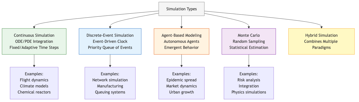
Continuous Simulation
State variables change continuously over time, governed by differential equations. Used in physics, control systems, and fluid dynamics.
- Time advances in fixed or adaptive steps
- Numerical solvers (Runge-Kutta, BDF) integrate ODEs/DAEs
- Examples: flight dynamics, chemical reactors, climate models
Discrete-Event Simulation (DES)
State changes occur at discrete points in time triggered by events. The simulation clock jumps from one event to the next.
- Event-driven time advancement
- Core data structure: priority queue of future events
- Examples: network packet routing, manufacturing lines, hospital workflows
Agent-Based Modeling (ABM)
Autonomous agents follow individual rules. System-level behavior emerges from local interactions.
- Each agent has state, perception, and decision logic
- Environment mediates interactions
- Examples: epidemic spread, market dynamics, urban growth
Hybrid Simulation
Combines two or more paradigms. A manufacturing plant might use DES for order flow, continuous simulation for thermal processes, and ABM for worker behavior.
┌─────────────────────────────────────┐
│          Hybrid Simulation          │
│  ┌─────────┐  ┌──────┐  ┌───────┐  │
│  │   DES   │◄─┤Bridge├─►│Contin.│  │
│  └─────────┘  └──┬───┘  └───────┘  │
│                  │                  │
│              ┌───▼───┐              │
│              │  ABM  │              │
│              └───────┘              │
└─────────────────────────────────────┘
Simulation Lifecycle
- Problem formulation — Define objectives, scope, and questions the simulation must answer.
- Conceptual modeling — Identify entities, relationships, assumptions, and simplifications.
- Data collection — Gather input parameters, distributions, and validation data.
- Model translation — Implement the conceptual model in code or a simulation platform.
- Verification — Confirm the code correctly implements the conceptual model.
- Validation — Confirm the model adequately represents the real system.
- Experimentation — Design and execute simulation runs (DOE, replications).
- Analysis — Interpret output using statistical methods.
- Documentation — Record assumptions, parameters, results, and limitations.
Model Abstraction
Abstraction controls fidelity vs computational cost. The right level depends on the questions being asked.
High Fidelity ◄──────────────────► High Abstraction
  CFD of airflow    │    Lumped thermal model
  Individual packets│    M/M/1 queue
  Molecular dynamics│    Continuum mechanics
Guidelines for abstraction level:
- Include only phenomena that affect outputs of interest
- Aggregate homogeneous entities (e.g., thousands of identical items become a flow rate)
- Replace complex subsystems with transfer functions when internal dynamics are irrelevant
- Use dimensional analysis to identify dominant terms
Verification and Validation
Verification ("Are we building the model right?")
Techniques:
- Code review and walkthroughs — Peer inspection of implementation
- Unit testing — Test individual components against known analytical solutions
- Trace analysis — Step through event sequences manually
- Degeneracy testing — Extreme inputs should produce expected extreme outputs
- Comparison with simplified models — A complex model under limiting conditions should match its simpler counterpart
Validation ("Are we building the right model?")
Techniques:
- Face validation — Domain experts judge plausibility
- Historical validation — Reproduce known past behavior
- Predictive validation — Forecast unseen data, compare with actuals
- Sensitivity-based validation — Model sensitivities should match observed real-system sensitivities
- Turing test — Experts cannot distinguish model output from real data
// Simple verification: compare simulation output to analytical result
PROCEDURE VERIFY_MM1_QUEUE(arrival_rate, service_rate, simulated_avg_wait) → boolean
    // Analytical: W_q = lambda / (mu * (mu - lambda)) for M/M/1
    rho ← arrival_rate / service_rate
    ASSERT(rho < 1.0, "System must be stable")
    analytical_wait ← arrival_rate / (service_rate * (service_rate - arrival_rate))
    relative_error ← ABS(simulated_avg_wait - analytical_wait) / analytical_wait
    RETURN relative_error < 0.05   // 5% tolerance
Sensitivity Analysis
Sensitivity analysis determines how variation in model inputs affects outputs. It identifies influential parameters and guides data collection effort.
One-at-a-Time (OAT)
Vary one parameter while holding others at baseline. Simple but misses interactions.
Global Methods
- Morris method (Elementary Effects) — Screen many parameters cheaply to rank importance
- Sobol indices — Decompose output variance into contributions from each parameter and their interactions
- First-order index S_i: fraction of variance due to parameter i alone
- Total-order index S_Ti: includes all interactions involving parameter i
- Latin Hypercube Sampling — Stratified sampling across parameter space for efficient coverage
Practical Workflow
1. Define parameter ranges and distributions
2. Generate sample points (LHS, Sobol sequence)
3. Run simulation at each sample point
4. Compute sensitivity indices
5. Rank parameters by influence
6. Focus validation effort on high-sensitivity parameters
Interpreting Results
| S_i ≈ S_Ti | Parameter has mostly direct effects |
|---|---|
| S_i << S_Ti | Parameter participates in strong interactions |
| S_Ti ≈ 0 | Parameter can be fixed without loss of accuracy |
Common Pitfalls
- Over-fitting the model — Adding detail beyond what data can support
- Ignoring warm-up bias — Including transient behavior in steady-state estimates
- Single replication — Drawing conclusions from one stochastic run
- Confusing verification with validation — Bug-free code can still model the wrong system
- Anchoring on a paradigm — Forcing DES when continuous or ABM would be more natural
When to Simulate
Simulation is justified when:
- The system does not yet exist (design exploration)
- Real experiments are too expensive, slow, or dangerous
- Analytical solutions are intractable
- Stochastic variability matters
- Interaction effects dominate and cannot be captured by closed-form models
Simulation is not justified when a simple analytical model suffices or when input data quality is too poor to produce meaningful results.