Speech Recognition (ASR)
Overview
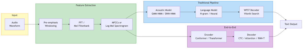
Automatic Speech Recognition (ASR) converts spoken language into text. The fundamental challenge: mapping a variable-length acoustic signal to a variable-length symbol sequence across diverse speakers, accents, noise conditions, and vocabularies.
Audio waveform -> Feature extraction -> Acoustic model -> Decoder -> Text
Traditional Pipeline: GMM-HMM
The dominant paradigm from the 1980s through ~2012.
Hidden Markov Models (HMMs)
Model temporal structure of speech at the phoneme level:
- States represent sub-phoneme units (typically 3 states per phoneme: beginning, middle, end)
- Transitions capture duration via self-loops and left-to-right topology
- Emission probabilities model acoustic observations at each state
Gaussian Mixture Models (GMMs)
Model the emission probability distribution at each HMM state:
p(x | state_j) = sum_{m=1}^{M} w_jm * N(x; mu_jm, Sigma_jm)
Typically 16-64 mixture components per state. Input: 39-dim MFCC + delta + delta-delta.
Training
- Baum-Welch (EM algorithm): Iteratively estimate GMM parameters and state alignments
- Viterbi training: Use best-path alignment instead of full forward-backward
- Decision tree clustering: Tie states across triphone contexts to handle data sparsity
- Discriminative training: MMI, MPE, sMBR objectives improve over maximum likelihood
Decoding
Viterbi search through the composed WFST (Weighted Finite-State Transducer):
Search graph = HMM * Context-dependency * Lexicon * Language Model
Beam search prunes the search space. The decoder finds the word sequence W that maximizes:
W* = argmax_W P(X|W) * P(W)^alpha * |W|^beta
Where alpha = language model weight, beta = word insertion penalty.
DNN-HMM Hybrid
Replace GMMs with deep neural networks (~2012 onward):
- DNN takes a context window of frames and predicts HMM state posteriors
- Convert to likelihoods via Bayes' rule: p(x|s) = p(s|x) * p(x) / p(s)
- HMM still handles temporal alignment and decoding
- Large improvement over GMMs, especially with deep architectures
Progression of acoustic models:
- DNN (feed-forward): Context window of ~11 frames
- RNN/LSTM: Process full sequence, capture long-range dependencies
- TDNN (Time-Delay Neural Network): Efficient temporal context via dilated 1D convolutions
- CNN-TDNN-LSTM: Combine complementary architectures
End-to-End Models
Eliminate the separate components (lexicon, pronunciation model, HMM) in favor of a single neural network that directly maps audio to text.
Connectionist Temporal Classification (CTC)
Maps input frames to output labels without requiring pre-aligned training data.
Key ideas:
- Output alphabet includes a blank token (for silence/repetition)
- All alignments that collapse to the same label sequence are marginalized:
"aaa-bb-" and "a--ab-b" both map to "ab"(where - is blank) - Forward-backward algorithm computes the total probability efficiently
- Conditional independence assumption: each frame's output is independent given the input
Limitations:
- Cannot model output dependencies (no implicit language model)
- Tends to produce peaky, spiky alignments
- Often combined with external language model in decoding
Used in: DeepSpeech, early wav2vec systems.
Attention-Based: Listen, Attend and Spell (LAS)
Encoder-decoder architecture with attention:
- Listener (encoder): Pyramidal BiLSTM reduces input sequence length
- Attention: Learns soft alignment between encoder states and output tokens
- Speller (decoder): Autoregressive LSTM generates characters/subwords
Advantages: Jointly learns alignment and language model. No conditional independence assumption.
Limitations: Attention-based alignment can fail on long utterances. Requires full input before decoding (not streaming-friendly without modifications).
RNN-Transducer (RNN-T)
Combines CTC-style frame processing with autoregressive label prediction:
- Encoder: Processes audio frames (like CTC)
- Prediction network: Processes previous labels (like a language model)
- Joint network: Combines both to predict next label or blank
- Supports streaming decoding (process audio left-to-right)
Dominant architecture for on-device ASR (Google, Apple). Handles the CTC conditional independence limitation while remaining streamable.
Conformer
State-of-the-art encoder architecture combining convolution and self-attention:
Input -> FeedForward -> Multi-Head Self-Attention -> Convolution -> FeedForward -> Output
- Self-attention captures global context
- Convolution captures local patterns
- Macaron-style feed-forward layers (half before, half after)
- Relative positional encoding
Used as the encoder in both CTC and RNN-T systems. Consistently outperforms pure Transformer or pure CNN encoders on speech tasks.
Whisper (OpenAI)
Large-scale weakly supervised ASR model:
- Architecture: Encoder-decoder Transformer (standard, no novel components)
- Training data: 680,000 hours of labeled audio from the internet
- Multitask: Transcription, translation, language ID, timestamp prediction via special tokens
- Input: 30-second mel-spectrogram chunks (80 mel bins, 16 kHz)
- Sizes range from Tiny (39M params) to Large-v3 (1.5B params)
Key insight: Scale and data diversity matter more than architectural innovation. Whisper achieves strong zero-shot performance across languages and domains without fine-tuning.
Distil-Whisper provides 6x faster inference with minimal accuracy loss.
Language Model Integration
External language models improve ASR output, especially for rare words and domain adaptation:
Shallow Fusion
Interpolate ASR and LM scores during beam search:
score = log P_ASR(y|x) + lambda * log P_LM(y)
Simple and effective. Works with any LM (n-gram, neural).
Deep Fusion and Cold Fusion
Integrate LM representations into the decoder at the hidden state level during training.
Rescoring
N-best list or lattice rescoring with a large LM after initial decoding. Allows using expensive models (GPT-scale) without slowing real-time decoding.
Evaluation: Word Error Rate (WER)
WER = (Substitutions + Insertions + Deletions) / Reference Words * 100%
Computed via dynamic programming alignment between hypothesis and reference.
| Metric | Description |
|---|---|
| WER | Standard word-level error rate |
| CER | Character Error Rate (useful for character-based languages) |
| SER | Sentence Error Rate (binary: any error in sentence) |
| RTF | Real-Time Factor: processing_time / audio_duration |
Benchmark datasets: LibriSpeech (English read speech), Common Voice (multilingual), Switchboard (conversational), GigaSpeech, FLEURS (multilingual).
Multilingual and Cross-Lingual ASR
Challenges
- Low-resource languages lack labeled training data
- Diverse phoneme inventories and tonal systems
- Writing system variation (alphabetic, logographic, abjad)
Approaches
- Multilingual pre-training: Train shared encoder on many languages, fine-tune on target
- Self-supervised learning: wav2vec 2.0, HuBERT, WavLM learn representations from unlabeled audio, then fine-tune with minimal labeled data
- Cross-lingual transfer: Phone-level representations transfer across related languages
- Whisper/MMS (Meta): Massively multilingual models covering 1,000+ languages
Self-supervised models (wav2vec 2.0, HuBERT) have dramatically reduced the labeled data requirements, enabling ASR for hundreds of previously unsupported languages.
Self-Supervised Pre-Training Pipeline
Unlabeled audio -> Encoder -> Contrastive/Masked prediction -> Pre-trained model
Fine-tune with CTC + small labeled dataset -> ASR system
wav2vec 2.0 achieves competitive WER on LibriSpeech with only 10 minutes of labeled data.