Algorithm Basics

An algorithm is a finite sequence of well-defined instructions for solving a problem or performing a computation. This file covers the foundational concepts for reasoning about algorithms.

What is an Algorithm?

Formal Properties

1. Input: Zero or more well-defined inputs.
2. Output: One or more well-defined outputs.
3. Definiteness: Each step is precisely defined (unambiguous).
4. Finiteness: Terminates after a finite number of steps.
5. Effectiveness: Each step is basic enough to be carried out in finite time.

Algorithm vs Program

An algorithm is an abstract concept — a method for solving a problem. A program is a concrete implementation of an algorithm in a specific programming language. The same algorithm can be implemented in many languages.

Correctness

Partial vs Total Correctness

Partial correctness: If the algorithm terminates, it produces the correct result.

Total correctness: Partial correctness + guaranteed termination.

Loop Invariants

A loop invariant is a property that holds:

1. Initialization: True before the first iteration.
2. Maintenance: If true before an iteration, it remains true after the iteration.
3. Termination: When the loop terminates, the invariant (combined with the exit condition) implies correctness.

Example: Insertion sort.

Invariant: At the start of iteration i, arr[0..i-1] is sorted and
           contains the same elements as the original arr[0..i-1].

Initialization: i=1, arr[0..0] is trivially sorted. ✓
Maintenance: Iteration i inserts arr[i] into the correct position
             in arr[0..i-1], resulting in sorted arr[0..i]. ✓
Termination: i=n, so arr[0..n-1] is sorted. ✓

Proving Termination

Show that a variant function (loop variant) — a non-negative integer quantity — strictly decreases with each iteration. Since it can't decrease below 0, the loop must terminate.

Example: Binary search. Variant = high - low. Each iteration, either low increases or high decreases, so the variant strictly decreases.

Algorithm Specification

Pseudocode

A human-readable description using a mix of natural language and programming constructs. Not tied to any language.

INSERTION-SORT(A, n)
    for i = 1 to n-1
        key = A[i]
        j = i - 1
        while j >= 0 and A[j] > key
            A[j+1] = A[j]
            j = j - 1
        A[j+1] = key

Describing Algorithms

Good algorithm descriptions include:

1. Input/output specification: What is given, what is produced.
2. High-level idea: Intuition behind the approach.
3. Detailed steps: Pseudocode or precise natural language.
4. Correctness argument: Why it works (invariant, induction, or informal reasoning).
5. Complexity analysis: Time and space bounds.

Algorithm Properties

Deterministic vs Nondeterministic

Deterministic: Same input always produces the same sequence of steps and output. Most algorithms are deterministic.

Nondeterministic: May make arbitrary choices at certain steps. Used in complexity theory (NP = nondeterministic polynomial time). Randomized algorithms use controlled randomness.

In-Place vs Out-of-Place

In-place: Uses O(1) extra memory (modifies input directly). Examples: insertion sort, quicksort (with in-place partition).

Out-of-place: Requires additional memory proportional to input size. Examples: merge sort (O(n) extra), hash table construction.

Stable vs Unstable (for Sorting)

Stable: Equal elements maintain their relative order from the input. Important when sorting by multiple keys.

Stable sorts: Insertion sort, merge sort, Timsort, counting sort, radix sort. Unstable sorts: Quicksort, heapsort, selection sort.

Online vs Offline

Online: Processes input piece by piece as it arrives. Must make decisions without seeing future input. Examples: insertion sort (can sort as elements arrive), LRU cache.

Offline: Has access to the entire input before processing. Examples: merge sort, optimal page replacement.

Adaptive

An adaptive algorithm performs better when the input is partially sorted (or has other structure).

Adaptive: Insertion sort (O(n) for nearly sorted), Timsort, natural merge sort. Non-adaptive: Heapsort (always O(n log n) regardless of input order).

Complexity Measures

Time Complexity

The number of basic operations (comparisons, assignments, arithmetic) as a function of input size n.

Best case: Minimum operations over all inputs of size n. Worst case: Maximum operations — the standard measure. Average case: Expected operations over a distribution of inputs. Amortized: Average over a worst-case sequence of operations.

Space Complexity

The amount of additional memory used (beyond the input).

In-place: O(1) extra space. Linear space: O(n) extra. Note: Recursive algorithms use O(depth) stack space.

Asymptotic Notation

• O(f(n)): Upper bound (worst case grows no faster than f).
• Ω(f(n)): Lower bound (best case grows no slower than f).
• Θ(f(n)): Tight bound (grows at the same rate as f).
• o(f(n)): Strict upper bound (grows strictly slower).
• ω(f(n)): Strict lower bound (grows strictly faster).

Detailed treatment in topic 17 (Algorithm Analysis).

Algorithm Design Paradigms

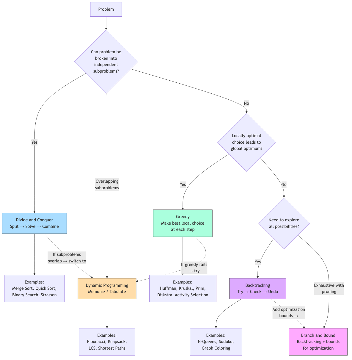
| Paradigm | Key Idea | Examples | |---|---|---| | Brute force | Try all possibilities | Exhaustive search, naive string matching | | Divide and conquer | Split, solve recursively, combine | Merge sort, quicksort, FFT | | Greedy | Make locally optimal choices | Dijkstra, Huffman, Kruskal | | Dynamic programming | Store and reuse subproblem solutions | Knapsack, LCS, shortest paths | | Backtracking | Explore, prune infeasible branches | N-queens, Sudoku, constraint satisfaction | | Randomized | Use randomness for efficiency/simplicity | Quicksort (random pivot), Miller-Rabin | | Approximation | Near-optimal solution in polynomial time | Vertex cover 2-approx, TSP 1.5-approx |

Each paradigm is covered in detail in subsequent files.

Problem-Solving Strategy

1. Understand the problem: Read carefully. Identify inputs, outputs, constraints.
2. Work through examples: Small cases by hand. Edge cases.
3. Identify the paradigm: Does it have optimal substructure (DP/greedy)? Can it be divided (D&C)? Is it a search problem (backtracking)?
4. Design the algorithm: Start with brute force, then optimize.
5. Prove correctness: Loop invariant, induction, or informal argument.
6. Analyze complexity: Time and space.
7. Implement: Translate to code. Handle edge cases.
8. Test: Verify with examples, edge cases, stress tests.

Applications in CS

• Software engineering: Algorithm choice directly impacts system performance, scalability, and resource usage.
• Interviews: Algorithm design and analysis is the core of technical interviews.
• Competitive programming: Fast problem-solving requires fluency in algorithm paradigms.
• Systems design: Understanding algorithmic tradeoffs (time vs space, exact vs approximate) informs architecture decisions.