Uninformed Search

Uninformed (blind) search strategies explore the state space without domain-specific knowledge about which states are closer to the goal.

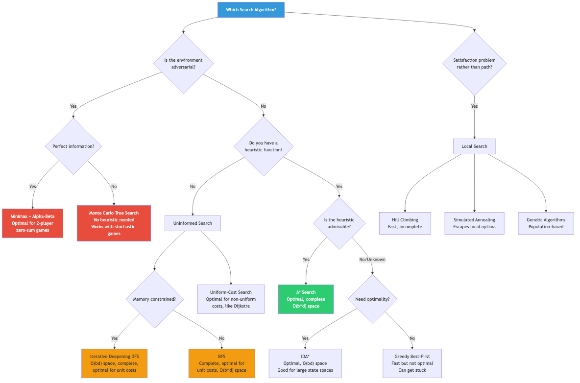
Problem Formulation

State space: Set of all possible states. Initial state: Starting point. Actions: Available moves at each state. Transition model: Result of applying an action. Goal test: Is this a goal state? Path cost: Cost of a path (sum of action costs).

Search Tree vs Search Graph

Tree search: May revisit states (explore the same state multiple times). Simpler but potentially exponential blowup.

Graph search: Track visited states (closed set). Never revisit. Uses more memory but avoids infinite loops and redundant work. Preferred in practice.

BFS (Breadth-First Search)

Explore nodes in FIFO order — all nodes at depth d before any at depth d+1.

PROCEDURE BFS(start, goal) → path or NONE
    queue ← empty FIFO queue
    visited ← empty set
    ENQUEUE(queue, (start, empty_path))
    ADD start TO visited

    WHILE queue IS NOT empty DO
        (state, path) ← DEQUEUE(queue)
        IF goal(state) THEN RETURN path
        FOR EACH (action, next) IN SUCCESSORS(state) DO
            IF next NOT IN visited THEN
                ADD next TO visited
                new_path ← path + [action]
                ENQUEUE(queue, (next, new_path))
    RETURN NONE

Property	Value
Complete?	Yes (if branching factor b is finite)
Optimal?	Yes (if all step costs are equal)
Time	O(b^d) where d = depth of shallowest goal
Space	O(b^d) — stores entire frontier

Space is the bottleneck: At b=10, d=10: ~10¹⁰ nodes. BFS is impractical for deep goals.

DFS (Depth-First Search)

Explore the deepest unexpanded node first. Uses a stack (or recursion).

Property	Value
Complete?	No (infinite paths). Yes with graph search on finite graphs.
Optimal?	No (may find a deep solution before a shallow one)
Time	O(b^m) where m = maximum depth
Space	O(bm) — only stores current path + siblings

Advantage: O(bm) space — dramatically less than BFS.

Uniform-Cost Search (UCS)

Expand the node with the lowest path cost g(n). Uses a priority queue.

Property	Value
Complete?	Yes (if step costs ≥ ε > 0)
Optimal?	Yes
Time	O(b^(1 + ⌊C/ε⌋)) where C = optimal cost
Space	Same as time

UCS is BFS generalized to weighted graphs. Equivalent to Dijkstra's algorithm.

Depth-Limited Search

DFS with a depth limit L. Avoids infinite paths. Incomplete if L < d (goal depth).

Iterative Deepening DFS (IDDFS)

Run depth-limited DFS with limits 0, 1, 2, 3, ... until the goal is found.

PROCEDURE IDDFS(start, goal) → path or NONE
    FOR depth_limit ← 0, 1, 2, ... DO
        result ← DLS(start, goal, depth_limit)
        IF result IS NOT NONE THEN
            RETURN result
    RETURN NONE

Property	Value
Complete?	Yes
Optimal?	Yes (uniform step costs)
Time	O(b^d) — same as BFS
Space	O(bd) — same as DFS!

Combines the best of BFS (completeness, optimality) and DFS (space efficiency). The repeated work is bounded by a constant factor: (b/(b-1))². For b=10: only 11% overhead.

IDDFS is the preferred uninformed search for most problems.

Bidirectional Search

Search simultaneously from the start and goal, meeting in the middle.

Time: O(b^(d/2)) — exponential improvement! Space: O(b^(d/2)).

Requirement: Must be able to search backward (know the goal state, generate predecessors). Checking intersection of two frontiers must be efficient (hash set).

Comparison

Algorithm	Complete	Optimal	Time	Space
BFS	Yes	Yes*	O(b^d)	O(b^d)
DFS	No	No	O(b^m)	O(bm)
UCS	Yes	Yes	O(b^(1+C*/ε))	Same
DLS	No	No	O(b^L)	O(bL)
IDDFS	Yes	Yes*	O(b^d)	O(bd)
Bidirectional	Yes	Yes*	O(b^(d/2))	O(b^(d/2))

(*with uniform step costs)

Applications in CS

Pathfinding: Grid-based navigation (games, robotics) when no heuristic is available.
Puzzle solving: 8-puzzle, 15-puzzle, Rubik's cube (BFS/IDDFS for optimal solutions).
Web crawling: BFS from seed URLs to discover web pages.
Network analysis: BFS for shortest paths in unweighted graphs, connected components.
Version control: Git uses graph search for merge-base finding, reachability.